Bilinear transformation

The bilinear transformation is the substitution

$$s=\frac{2(z-1)}{z+1}$$

used to convert the representation of a continuous (or "analog") system into the representation of a discrete (or "digital") system.

For example, the second order low pass Butterworth filter with cutoff frequency ω_c is usually given by the Laplace transform transfer function

$$H(s)=\frac{\omega_c^2}{s^2+\sqrt{2}\omega_cs+\omega_c^2}$$

With the bilinear transformation, the Z transform transfer function of the same filter is

$$H(\frac{2(z-1)}{z+1})=\frac{\omega_c^2}{(\frac{2(z-1)}{z+1})^2+\sqrt{2}\omega_c^2\frac{2(z-1)}{z+1}+\omega_c^2}$$ $$=\frac{\omega_c^2+2\omega_c^2z^{-1}+\omega_c^2z^{-2}}{(4+2\sqrt{2}\omega_c+\omega_c^2)+(-8+2\omega_c^2)z^{-1}+(4-2\sqrt{2}\omega_c+\omega_c^2)z^{-2}}$$

Scaling to obtain 1 in the denominator, we have

$$H(z) = \frac{a_0+a_1z^{-1}+a_2z^{-2}}{1+b_1z^{-1}+b_2z^{-2}}$$ $$a_0=a_2=\frac{\omega_c^2}{4+2\sqrt{2}\omega_c+\omega_c^2}$$ $$a_1=\frac{2\omega_c^2}{4+2\sqrt{2}\omega_c+\omega_c^2}$$ $$b_1=\frac{-8+2\omega_c^2}{4+2\sqrt{2}\omega_c+\omega_c^2}$$ $$b_2=\frac{4-2\sqrt{2}\omega_c+\omega_c^2}{4+2\sqrt{2}\omega_c+\omega_c^2}$$

and the impulse response of the filter (its actual implementation in practice) is

$$y(k)=a_0x(k)+a_1x(k-1)+a_2x(k-2)-b_1y(k-1)-b_2y(k-2)$$

where x(n) are the samples of the input signal and y(n) are the samples of the output signal.

Derivation of the bilinear transformation

The bilinear transformation follows from the Taylor series expansion of the function e^sT/2.

$$z=e^{sT}=\frac{1+\frac{(\frac{sT}{2})^1}{1!}+\frac{(\frac{sT}{2})^2}{2!}+...}{1+\frac{(-\frac{sT}{2})^1}{1!}+\frac{(-\frac{sT}{2})^2}{2!}+...}\approx\frac{1+\frac{sT}{2}}{1-\frac{sT}{2}}$$

Frequency warping of the bilinear transformation

Note that the properties of the resulting filter are evaluated at s = jω or z = e^jω. However,

$$H(s)=H(j\omega)$$ $$H(\frac{2(z-1)}{z+1})=H(\frac{2(e^{j\omega}-1)}{e^{j\omega}+1})=H(2\frac{e^{\frac{j\omega}{2}}(e^{\frac{j\omega}{2}}-e^{-\frac{j\omega}{2}})}{e^{\frac{j\omega}{2}}(e^{\frac{j\omega}{2}}+e^{-\frac{j\omega}{2}})})$$ $$=H(2\frac{2jsin(\frac{\omega}{2})}{2cos(\frac{\omega}{2})})=H(2j\,tan(\frac{\omega}{2}))$$

Thus, the discrete filter H(z), obtained after the bilinear transformation of H(s), will behave, at the discrete frequency ω_d, the same way the continuous filter H(s) behaves at the frequency ω_a = 2 tan(ω_d/2). (Alternatively, ω_d = 2 arctan(ω_a/2)).

Take, for example, the Butterworth filter above. Its magnitude response, computed from H(s), is

$$|H(j\omega)H(-j\omega)|=\sqrt{\frac{\omega_c^4}{\omega^4+\omega_c^4}}$$

The magnitude response of the filter after the bilinear transformation can be computed from

$$H(z)=\frac{\omega_c^2z+2\omega_c^2+\omega_c^2z^{-1}}{(4+2\sqrt{2}\omega_c+\omega_c^2)z+(-8+2\omega_c^2)+(4-2\sqrt{2}\omega_c+\omega_c^2)z^{-1}}$$

and is

$$|H(e^{j\omega})H(e^{-j\omega})|=\sqrt{\frac{\omega_c^4(cos(\omega)+1)^2}{\omega_c^4(cos(\omega)+1)^2+16(cos(\omega)+1)^2-64cos(\omega)}}$$ $$=\sqrt{\frac{\omega_c^4}{\omega_c^4+16\frac{(cos(\omega)-1)^2}{(cos(\omega)+1)^2}}}=\sqrt{\frac{\omega_c^4}{\omega_c^4+(2tan(\frac{\omega}{2}))^4}}$$

This warping of the frequency domain is small for small ω and increases as ω increases (ω is between 0 and π). At ω_a = 1, for example, ω_d ≈ 0.927.

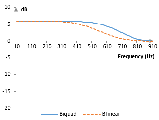
When designing digital filters, this frequency warping can be remedied in one of two ways. First, a discrete filter with the cutoff frequency ω_d can be designed with the bilinear transformation on the continuous filter with the cutoff frequency ω_a = 2 tan(ω_d/2). Alternatively, instead of the bilinear transformation, one can use the biquad transformation

$$s=\frac{1}{K}\frac{z-1}{z+1}, \, K=tan(\frac{\omega_c}{2})$$

For example, the second order low-boost shelving filter with cutoff frequency ω_c and gain G

$$H(s)=\frac{s^2+\sqrt{2G}\omega_cs+G\omega_c^2}{s^2+\sqrt{2}\omega_cs+\omega_c^2}$$

can be written with the bilinear transformation as

$$H(z)=\frac{(4+2\sqrt{2G}\omega_c+G\omega_c^2)+(-8+2G\omega_c^2)z^{-1}+(4-2\sqrt{2G}\omega_c+G\omega_c^2)z^{-2}}{(4+2\sqrt{2}\omega_c+\omega_c^2)+(-8+2\omega_c^2)z^{-1}+(4-2\sqrt{2}\omega_c+\omega_c^2)z^{-2}}$$

or with the biquad transform as

$$H(z)=\frac{(1+\sqrt{2G}K+GK^2)+(-2+2GK^2)z^{-1}+(1-\sqrt{2G}K+GK^2)z^{-2}}{(1+\sqrt{2}K+K^2)+(-2+2K^2)z^{-1}+(1-\sqrt{2}K+K^2)z^{-2}}$$

The corresponding magnitude responses for the example cutoff frequency ω_c = 2 in both cases, K = tan(ω_c / 2), sampling rate of 2000 Hz, and gain of G = 2 (≈ 6 dB) are below.

Filter stability and the bilinear transformation

Note that, for s = σ + j ω, if Re(s) = σ < 0, then

$$|z|=|\frac{2+s}{2-s}|=|\frac{2+\sigma+j\omega}{2+\sigma-j\omega}|=\frac{|2+\sigma+j\omega|}{|2-\sigma-j\omega|}$$ $$=\frac{\sqrt{(2+\sigma)^2+\omega^2}}{\sqrt{(2-\sigma)^2+\omega^2}}\lt1$$

Thus, if we have the Laplace transform transfer function of a stable filter with roots of the denominator in the left part of the s- complex plane, the transfer function that we will obtain with the bilinear transformation would have roots that are inside the unit circle and the filter will still be stable. The bilinear transformation preserves stability.