Haar wavelet transform

A definition of the Haar wavelet transform is provided below. There are many ways to define the transform. The definition here is derived from the following example decomposition of a short audio signal.

Example level eight Haar wavelet transform of a signal

Consider the following example signal.

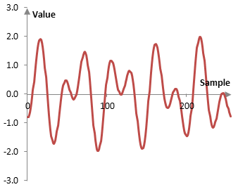
This example signal is the sum of two simple sine waves, one with a frequency of 5 Hz and phase of zero (i.e., the wave starts with the value zero at sample zero) and one with a frequency of 9 Hz and shifted to the right by 10 samples. The sampling frequency is 256 Hz and the graph above shows 256 samples (1 second) of the signal.

Denote the value of this signal at sample k with x(k). Let K = 256 and, for 1 second of time, k = 0, 1, …, K – 1. Compute

$$a_1(j)=\frac{x(k-1)+x(k)}{\sqrt{2}}$$ $$b_1(j)=\frac{x(k-1)-x(k)}{\sqrt{2}}$$

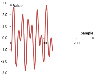
for j = 0, 1, …, K/2 and k = 2j + 1. The computed signal a₁(j) is a moving average of x(k). It smooths out the signal x(k), removing some of the variability between two adjacent samples. It also compresses the signal x(k) in time. The signal b₁(j) contains the fluctuations that the signal a₁(j) removes. The following is a plot of a₁(j).

Note the following.

• x(k) can be reconstructed from the signals a₁(j) and b₁(j)

$$x(k-1)=\frac{a_1(j)+b_1(j)}{\sqrt{2}}$$ $$x(k)=\frac{a_1(j)-b_1(j)}{\sqrt{2}}$$

• a₁(j) and b₁(j) preserve the energy of the signal x(k) (except for precision issues related to the quantization; see Dithering), in the sense that

$$a_1(j)^2+b_1(j)^2=x(k-1)^2+x(k)^2$$

• Often, many of the values of b₁(j) are relatively small. This fact is used below. In principle, according to the Nyquist-Shannon sampling theorem, a discrete signal sampled at the sampling frequency of fs represents frequencies between 0 and fs/2. Fluctuations will be larger only if the signal contains higher frequencies. Only frequencies above fs/4 with peak amplitude of 1, for example, will contain fluctuations larger than 1.

The transformation x(k) → (a₁(j) | b₁(j)) is the Haar wavelet transform of level 1. To compute the Haar wavelet transform of level 2, we take the Haar wavelet transform of level 1 of the signal a₁(j).

• If the signal x(k) is of length K, then the signal a₁ is of length K/2, and the signal a₂ is of length K/4.
• The energy of a₁ is preserved in a₂ and b₂.
• a₁ can be reconstructed similarly to above from a₂ and b₂. Then x(k) can be reconstructed from a₂, b₂, and b₁. The level 2 Haar wavelet transform can then be denoted by x → (a₂ | b₂ | b₁).

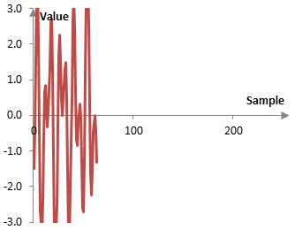
The following is a plot of our example a₂, which compresses the signal even further.

Since our example signal is of 256 discrete points, this process can be continued to level 8. At level 8, a₈ and b8 will each consist of a single point. The signal will be compressed to one point.

Definition of the Haar wavelet transform

Given a signal x(k) of length K = 2^N, for some integer N, the level N Haar wavelet transform of x(k) is (a_N | b_N | b_N-1 | … | b₁), where

$$a_1(j)=\frac{x(k-1)+x(k)}{\sqrt{2}}$$ $$b_1(j)=\frac{x(k-1)-x(k)}{\sqrt{2}}$$

j = 0, 1, …, K/2 and k = 2j + 1, and

$$a_n(i)=\frac{a_{n-1}(j-1)+a_{n-1}(j)}{\sqrt{2}}$$ $$b_n(i)=\frac{a_{n-1}(j-1)-a_{n-1}(j)}{\sqrt{2}}$$

n = 2, 3, …, N; i = 0, 1, …, K / 2ⁿ; and j = 2i + 1.

We note that, as before,

$$x(k-1)=\frac{a_1(j)+b_1(j)}{\sqrt{2}}$$ $$x(k)=\frac{a_1(j)-b_1(j)}{\sqrt{2}}$$ $$a_{n-1}(j-1)=\frac{a_n(i)+b_n(i)}{\sqrt{2}}$$ $$a_{n-1}(j)=\frac{a_n(j)-b_n(j)}{\sqrt{2}}$$

Haar wavelets

An alternative way to produce a similar result is to compute the inner product of the signal x(k) with the set of functions described below. To calculate a_N in the definition above, which is a single number, calculate the inner product of x(k) and

$$\psi^a_N (k)=\frac{1}{2^{\frac{N-1}{2}}}$$

We use the superscript "a" to show that these functions are used to compute the "a" portion of the Haar wavelet transform. Use the following two functions to calculate a^N-1, which is a vector of two values.

$$\psi^a_{N-1} (k)=\begin{cases} (-1)^m \frac{1}{2^{\frac{N-1}{2}}}, m \frac{K}{2} \le k \lt (m+1) \frac{K}{2} \\ 0, k \lt m \frac{K}{2}, k \ge (m+1) \frac{K}{2} \end{cases}, m=0,1$$

More generally, a_N-n for the N – n level of the transform can be calculated with the 2ⁿ functions (n=0, 1, …, N)

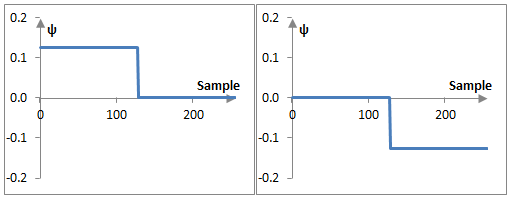
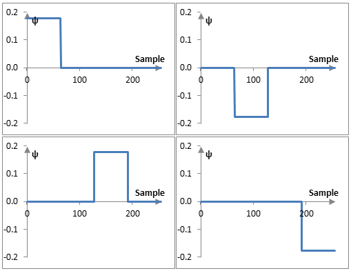
$$\psi^a_{N-n} (k)=\begin{cases} (-1)^m \frac{1}{2^{\frac{N-(n+1)}{2}}}, m \frac{K}{2^n} \le k \lt (m+1) \frac{K}{2^n} \\ 0, k \lt m \frac{K}{2^n}, k \ge (m+1) \frac{K}{2^n} \end{cases}, m= 0,1,...,2^n-1$$

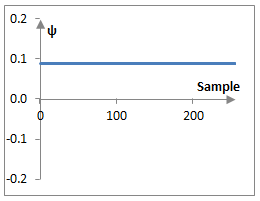
To understand this result, consider the following plots of ψ^a₈, ψ^a₇, and ψ^a₆ in the example above

It is only slightly more cumbersome to derive similar functions to compute the values of b. For example,

$$\psi^b_{1} (k)=\begin{cases} (-1)^k \frac{1}{2^{\frac{1}{2}}}, m \frac{K}{2^{N-1}} \le k \lt (m+1) \frac{K}{2^{N-1}} \\ 0, k \lt m \frac{K}{2^{N-1}}, k \ge (m+1) \frac{K}{2^{N-1}} \end{cases}, m= 0,1,...,2^{N-1}-1$$ $$\psi^b_{2} (k)=\begin{cases} (-1)^{int(\frac{k}{2})} \frac{1}{2^{\frac{2}{2}}}, m \frac{K}{2^{N-2}} \le k \lt (m+1) \frac{K}{2^{N-2}} \\ 0, k \lt m \frac{K}{2^{N-2}}, k \ge (m+1) \frac{K}{2^{N-2}} \end{cases}, m= 0,1,...,2^{N-2}-1$$ $$...$$ $$\psi^b_{n} (k)=\begin{cases} (-1)^{int(\frac{k}{2^{n-1}})} \frac{1}{2^{\frac{n}{2}}}, m \frac{K}{2^{N-n}} \le k \lt (m+1) \frac{K}{2^{N-n}} \\ 0, k \lt m \frac{K}{2^{N-n}}, k \ge (m+1) \frac{K}{2^{N-n}} \end{cases}, m= 0,1,...,2^{N-n}-1$$

n = 1, 2, …, N. Switch n and N-n in the last formula to obtain a result that is more consistent with the definition of ψ^a. The plots of ψ^b are very similar to the plots of ψ^a.

These types of functions are often defined more generally (and in the case of continuous time) with

$$\psi(x)=\begin{cases} 1, 0 \le x \lt \frac{1}{2} \\ -1, \frac{1}{2} \lt x \le 1 \\ 0, x=\frac{1}{2}, x \lt 0, x \gt 1 \end{cases}$$ $$\psi_{n,m}=\psi(2^n x - m)$$

for the integers n = 0,1, … and m=0, 1, …, 2ⁿ-1. These are the Haar wavelets. ψ(x) is known as the mother wavelet. Setting the value ψ(0.5) = 0 has its disadvantages, but that is beyond the scope of this topic.

These functions are orthogonal, since

$$\int_0^1 \psi(x) \, \psi_{n,m}(x) \, dx=0, \, (n,m) \ne (0,0)$$ $$\int_0^1 \psi_{i,j}(x) \, \psi_{n,m}(x) \, dx=0, \, (n,m) \ne (i,j)$$

These functions would become orthonormal, if we define instead

$$\psi_{n,m}=2^n \, \psi(2^n\,x-m)$$

This definition is very common, although it is not immediately obvious from this definition how to use the Haar wavelets in the Haar wavelet transform.

Using the Haar wavelet transform: data compression and noise reduction

The fact that many of the values computed with the Haar wavelet transform are small means that the transform can be used to compress the amount of data used.

Specifically, in the example above, there are 256 values that represent the Haar wavelet transform of the signal: 128 values for b₁, 64 values for b₂, …, 2 values for b₇, one value for b₈, and one value for a₈. To achieve 2:1 compression, we can simply remove the smallest 128 values and assume they are zero (i.e., zero them out and transmit only the remaining "nonzero" amounts). If we are to transmit these data, we would only have to transmit 128 values instead of 256, plus several bytes that detail the position of the nonzero values in the original signal (e.g., we can use 32 bytes or 8 four-byte integers to describe whether each of the 256 values is zero or not).

If we are to reconstruct the resulting signal from the compressed Haar wavelet transform, we would get the following.

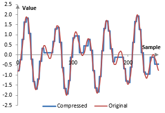
Of course, compression of only 2:1 is not impressive and one can even achieve a similar ratio with compression techniques that do not lose information. We can, however, obtain even higher compression rations, if we are willing to sacrifice some more of the precision. We can also achieve higher compression rations with more powerful wavelets than the Haar wavelet. The same method can also be used for removing low-level random noise from the signal.