Pitch shifting - part 1

We will deconstruct a pitch shift, since it is one of the more complex processing of digital audio. We will use the Fourier transform to detect frequencies. We will then pitch shift these frequencies and construct the pitch shifted signal.

We will use the following setup:

• Sampling rate of 2000 Hz: A small sampling rate makes charts easy.
• Discrete Fourier Transform (DFT) of 32 samples: Even though the DFT can use any length, a typical audio processor would use the Fast Fourier Transform algorithm, which requires a length equal to some power of 2.
• DFT overlap of 75 percent: We cannot take the DFT of the whole signal and will have to do it in pieces (segments or frames). To ensure a smooth result, these segments will overlap. We will discuss overlap more later.
• Incoming frequency of 70 Hz: There is nothing special here, but it is good to note two things. First, we are working with a signal of one frequency. Realistic signals will have multiple frequencies. The computations though are the same. Second, if the sampling rate is 2000 Hz and the DFT has 32 samples (or "bins"), then the DFT bins are 2000/32 = 62.5 Hz apart. Thus, 70 Hz is not on a DFT bin. Pitch shifting a frequency that is not on a DFT bin shows some of the problems of DFT that a frequence on the bin would not show.
• Pitch shift of 1.0594: Again, there is nothing special here, other than the fact that one semitone is 2^1/12 = 1.0594. We will pitch shift 70 Hz by one semitone, to about 74.2 Hz.
• Windowing: We will use the Hann window both during the deconstruction of the signal with the DFT and during the construction of the new signal with the inverse DFT. We will write more about this later.

Incoming signal

The incoming sampled signal in this exercise is simply

$$f(k) = cos(\frac{2 \pi k 70}{2000})$$

where k are the samples (k = 0, 1, 2, …), 70 is the signal frequency, and 2000 is the sampling frequency.

We are only putting this formula here in case someone wants to replicate this exercise. We will not be listing formulae for well-known computations, such as the DFT.

Here are the first 32 samples of the signal.

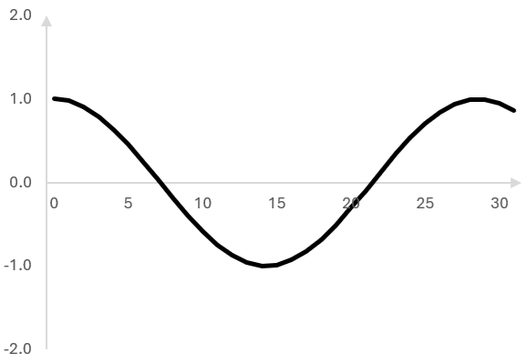
The signal can, of course, continue indefinitely.

Decomposition with the DFT

Using the 32-sample DFT on these 32 samples, we can compute that each of the frequencies on the DFT bins have the following magnitudes.

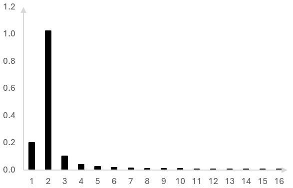
The x-axis shows the first half of the DFT bins. We show only half of the DFT and not all 32 bins. The second half of the DFT on a real valued signal will produce identical values and is redundant.

Since 70 Hz is not on a DFT bin, there is spectral leakage. We have magnitudes at each bin, even though we are using a signal of only one frequency. This will not hinder our pitch shift, as we will use all available info and work with all bins.

This graph is not surprising. 70 Hz is close to the second bin of the DFT at 62.5 Hz and most of the magnitude shows up there.

The DFT also produces the phase of the frequency at each bin. Those phases are extremely important, and we will discuss them later.

We will call the first 32 samples the first frame. In recorded audio, the signal will change over time. We cannot simply rely on the first 32 samples. We will have to take the DFT not just of the first 32 samples, but of the next ones and the next ones and so on until we know the composition of the whole signal over time. Thus, we will be working frame by frame.

Windowing with the Hann window

We computed the DFT of the signal as is, but it is better to apply a window to the signal first. Let's do so and recompute the DFT.

We will use the Hann window of 32 samples and will multiply the signal values at each sample by the window values at that sample.

Here is the windowed signal (solid line) next to the original signal (dotted line).

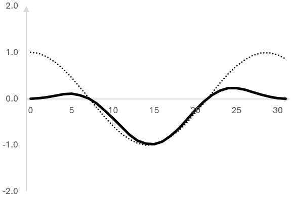
The Hann window compresses the left and right side of the signal frame.

We take the DFT of this new signal, but we also:

• Drop the first bin of the DFT (the zero frequency DC bin), by zeroing out its magnitude. The Hann window can exacerbate DC values and can shift the pitch shifted signal.
• Scale the resulting magnitudes by the coherent gain of the Hann window. By compressing the sides of the signal, the Hann window reduces the magnitude of the signal by that coherent gain. The coherent gain is just the average of the Hann window values and, for the Hann window, is approximately 0.5 (i.e., we divide by 0.5).

Here are the magnitudes of the DFT bin as originally computed, without the window (dotted bars) and with the window (solid bars).

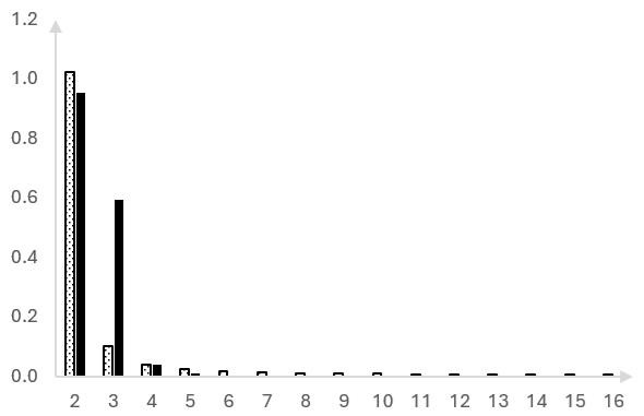
This looks worse perhaps. The original magnitude peak has now spread into two bins.

But zoom into the bins further out.

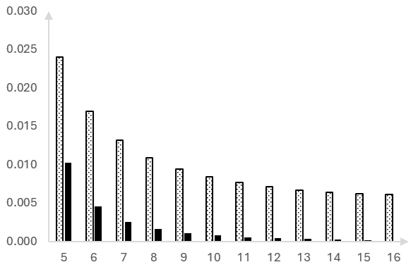
The window has, in fact, pushed the magnitudes that "leaked" into higher bins back towards the lower bins, closer to the input frequency of 70 Hz.

Next steps

This is the first step: decomposing the original signal into a set of magnitudes and phases. In the next post, we will compute the magnitudes and phases of the pitch shifted signal. With the last step, we will construct the new, pitch shifted signal.

authors: mic