Three different Fourier transforms are usually defined and all have applications in digital signal processing.
The continuous Fourier transform of the function x(t) is defined with the formula
$$H(s)=\int_{-\infty}^{\infty} x(t) \, e^{-2\pi\,j\,t\,s} \, dt$$
The inverse continuous Fourier transform is
$$x(t)=\int_{-\infty}^{\infty} H(s) \, e^{2\pi\,j\,t\,s} \, ds$$
The discrete Fourier transform of the function x(k) is defined with the formula
$$H(n)=\sum_{k=0}^{N-1} x(k) \, e^{-\frac{2\pi\,j\,k\,n}{N}}, \, n=0,1,...,N-1$$
and its inverse is
$$x(k)=\frac{1}{N}\sum_{n=0}^{N-1} H(n) \, e^{\frac{2\pi\,j\,k\,n}{N}}, \, k=0,1,...,N-1$$
The discrete-time Fourier transform is defined by the formula
$$H(s)=\sum_{k=-\infty}^{\infty} x(k) \, e^{-2\pi\,s\,j\,k}$$
and its inverse, usually written using ω = 2π f, is
$$x(k)=\frac{1}{2\pi}\int_{-\pi}^{\pi} H(\omega) \, e^{j\,\omega\,k} \, d\omega$$
The three forms of the Fourier transform above are sometimes abbreviated as FT, DFT, and DTFT.
Interpretation of the Fourier transform
As any other transform, the Fourier transform translates one type of function into another. The usual interpretation of the Fourier transform in digital signal processing is that the Fourier transforms translate a signal – a function of time and with values the signal values given specific amplitudes, frequencies, and phase amounts – into a function of frequencies that produces the amplitudes and phases of these frequencies given a specific time.
Typically, we define the signal x(t) as the sum of simple sine and cosine waves as follows.
$$x(t)=\sum_{n=0}^{N-1} A_n \, \cos(2\pi\,f_n\,(t-\tau_n))$$
where fn, An, and τ n are respectively the frequencies, amplitudes, and phases of these simple waves. This signal x(t) is a function of time for a set of predefined frequencies, amplitudes, and phases. The values of x(t) are the values of the signal.
The Fourier transform H(s) on the other hand is a function of the frequency s. H(s) itself has complex values, which, as shown below, contain information about the amplitudes and phases of the simple waves in the signal. Since the time t is not a part of the argument or values of H(s), the Fourier transform H(s) produces the amplitude and phase of the frequency s at a specific, predefined time t. The transform may produce different amplitudes and phases at different times t.
One more simplistic way of stating this is that, if we have a signal as a function of time, the Fourier transform can help us identify and analyze the amplitudes and phases of frequencies present in this signal.
The following helps explain this statement in the case of the discrete Fourier transform.
Take the discrete Fourier transform of a signal x(k) in discrete time k and apply Euler's formula.
$$H(n)=\sum_{k=0}^{N-1} x(k) \, e^{-\frac{2\pi\,j\,k\,n}{N}}$$ $$=\sum_{k=0}^{N-1} x(k) \, \cos(\frac{2\pi\,k\,n}{N})-j \sum_{k=0}^{N-1} x(k) \, \sin(\frac{2\pi\,k\,n}{N})$$
for n = 0, 1, …, N – 1. Suppose that x(k) is a real valued signal. Fourier analysis tells us that
$$\sum_{k=0}^{N-1} x(k) \, \cos(\frac{2\pi\,k\,n}{N}) \approx \frac{N B_n}{2}$$ $$\sum_{k=0}^{N-1} x(k) \, \sin(\frac{2\pi\,k\,n}{N}) \approx \frac{N C_n}{2}$$
where Bn = An cos(2π n τn) and Cn = An sin(2π n τn) are the coefficients of the simple wave An \cos(2π n (t - τn)) in x(k) with integer frequency n, amplitude An, and phase τn.
As explained in the topic Fourier analysis, the above result happens because simple waves are orthogonal and the sum products above produce a zero (approximately in the discrete case) for every such simple sine or cosine wave in x(k) except for the ones at n and at N – n.
$$H(n) \approx \frac{N\,B_n}{2}-j \frac{N\,C_n}{2}$$
Further, Bn and Cn can be used to compute the amplitude and phase
$$|A_n|=\sqrt{B_n^2+C_n^2}$$ $$\Phi_n=\mathrm{atan2}(\frac{C_n}{B_n})$$
of the frequency n in the signal x(k).
Simply put, H(n), the nth complex value of the Fourier transform, helps us find the amplitude An and phase Φn (through the coefficients Bn and Cn) of the simple wave with integer frequency n in the complex signal x(k).
In practice, we often have only a complex signal x(t) or x(k) and we do not know what frequencies comprise this signal. We can use the Fourier transform to find them. In the example above, the Fourier transform decomposes the real valued signal x(k), the signal values in time, into a set of amplitudes and phases H(n) for frequencies n.
In practice, there is also no guarantee that the complex signal x(t) or x(k) is composed of simple sine or cosine waves with integer frequencies (see, for example, Square wave). However, it can often be approximated by a sum of such simple waves, as discussed in the topic Fourier analysis.
Thus, the Fourier transform is a natural extension of the Fourier series. There are three motivations for using the Fourier transform rather than the Fourier series. First, the Fourier transform allows for shorter notation. Second, the use of complex numbers allows the Fourier transform to return a complex valued function, which means two separate values that can be used to describe the amplitude and the phase of the signal separately. Using complex numbers in the Fourier transform allows us to compute the coefficients Bn and Cn simultaneously and to produce a single function H(n) – a function that indirectly returns both amplitude and phase. Third, the Fourier transform has an inverse transform, which is easy to describe and which has its own uses.
Example – the discrete Fourier transform of a simple wave
Тake a simple discrete sine wave with frequency f, amplitude A and phase m, sampled over N points for a period of time 1. The values of this simple wave would be
$$A \, \sin(\frac{2\pi\,f\,(k-m)}{N})=B \, \cos(\frac{2\pi\,f\,k}{N})+C \, \sin(\frac{2\pi\,f\,k}{N})$$
where B = -A \sin(2π f m / N) and C = A \cos(2π f m / N). We can compute the discrete Fourier transform as follows.
$$H(n)=\sum_{k=0}^{N-1}(B \, \cos(\frac{2\pi\,f\,k}{N})+C \, \sin(\frac{2\pi\,f\,k}{N})) \, e^{-\frac{2\pi\,j\,k\,n}{N}}$$
for n = 0, 1, …, N – 1. We use Euler's formula again
$$e^{-\frac{2\pi\,j\,k\,n}{N}}=\cos(\frac{2\pi\,n\,k}{N})-j \, \sin(\frac{2\pi\,n\,k}{N})$$
and note that the components of the Fourier transform (the sine and cosine functions with frequency n) are orthogonal to the simple wave with frequency f over the sampling period, except in two cases – for n = f and for n = N – f. In the second case, we note that
$$\cos(\frac{2\pi\,n\,(N-k)}{N})=\cos(2\pi\,n-\frac{2\pi\,n\,k}{N})=\cos(\frac{2\pi\,n\,k}{N})$$ $$\sin(\frac{2\pi\,n\,(N-k)}{N})=\sin(2\pi\,n-\frac{2\pi\,n\,k}{N})=-\sin(\frac{2\pi\,n\,k}{N})$$
The transform, as a function of n, translates to
$$H(n) \approx \begin{cases} B \sum_{k=0}^{N-1} \cos^2 (\frac{2\pi\,k\,n}{N}) - j \, C \sin^2 (\frac{2\pi\,k\,n}{N}), \, n=f, N-f \\ 0, \,\, n \ne f, N-f\end{cases}$$
The two sums for a large enough sampling frequency N evaluate to approximately N / 2 and so the transform is simply
$$H(n) \approx \begin{cases} \frac{N}{2} (B - j \, C), \, n=f, N-f \\ 0, \,\, n \ne f, N-f\end{cases}$$
Thus, the discrete Fourier transform of a simple wave with frequency f produces a function H(n) that indicates something about the single wave at components n = f and n = N – f and is zero otherwise. Specifically, at n = f and n = N – f .
$$|H(n)| \approx \sqrt{Re(H(n))^2+Im(H(n))^2}=\frac{N}{2} \sqrt{B^2+C^2}=\frac{N}{2} A$$ $$\mathrm{atan2}(Im(H(n)),\,Re(H(n)))=\mathrm{atan2}(N C,\,N B)=-\frac{2\pi\,f\,m}{N}$$
These are the amplitude (scaled by N / 2) and phase of the original simple sine wave.
Example – discrete Fourier transform of a real valued complex signal
If the original wave is a complex real valued signal consisting of various waves with different amplitudes and frequencies, the result will be similar due to the fact that simple sine or cosine waves with different frequencies are orthogonal. Each component of the discrete Fourier transform (for each n) will produce the magnitude and phase of the corresponding simple wave (with frequency n) in the complex signal, if that wave is present in the complex signal.
The discrete Fourier transform H(n) of a real valued signal x(k), evaluated at the frequency n, shows the amplitude of the nth simple wave component in the signal x(k)
$$A_n=2 \frac{|H(n)|}{N}=2 \frac{\sqrt{Re(H(n))^2+Im(H(n))^2}}{N}$$
and the phase of the nth simple wave component in x(k)
$$\Phi_n=\mathrm{atan2}(Im(H(n),Re(H(n)))$$
It is important to note that the Fourier transform works because its components (the transform basis) and sine and cosine functions in general are orthogonal over properly selected intervals. In the ideal case, when a signal is composed only of waves with frequencies equal to those employed by the transform, the integrals or sums of the transform definition will produce zero in all cases except where a wave in the signal has the same frequency as the component of the transform. (In the less ideal case, where signal frequencies are not the same as those of the transform components, the result is less precise, but similar).
Redundant values of the Fourier transform of real valued signals
Suppose that we compute the discrete Fourier transform of a simple sine wave at 10 Hz, using the discrete Fourier transform with 100 points over 2 seconds of the wave. The magnitude of the resulting discrete Fourier transform components will be as in the following figure.
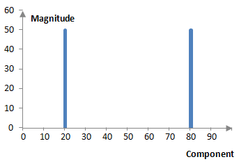
The discrete Fourier transform will be non-zero – approximately – at components 20 and 80. Since we are sampling with 100 points over 2 seconds, we have effectively sampled the wave with the sampling frequency 50 Hz. This means that we have used the discrete Fourier transform with components at 0.5 Hz, 1 Hz, 1.5 Hz, …, 49.5 Hz (These multiples of 0.5 Hz are orthogonal over 2 seconds.). The 20th component is 10 Hz and it makes sense that we have a non-zero value at this component. According to the discussion above, we also get a non-zero value at component 80 = 100 – 20. The magnitude of the discrete Fourier transform at these components is 100 / 2 = 50. These results are as expected. (We chose to compute the discrete Fourier transform with N uniform points over 2 seconds. How we choose the points of the discrete Fourier transform defines what the transform components are. In this case, the components represent the frequencies between 0 and N / 2. Most often, the discrete Fourier transform is computed with the first N points of a signal sampled at the sampling frequency fs. In this case, the components are the frequencies 0, fs / N, 2 fs / N, …, (N – 1) fs / N. The discrete Fourier transform then poses one interesting question, namely what the component at 0 represents. The magnitude of the component at 0 for a signal of the form x(k) = A0 + A1 sin(2π k f / N) would be N A0. Thus, although the discrete Fourier transform component at 0 is usually meaningless for digital signal processing, in analog signals it represents DC current.)
When the input to the discrete Fourier transform or the inverse discrete Fourier transform is real valued and not complex, the transform produces complex numbers such that H(N – 1 – n) is the complex conjugate of H(n). The information for n > N / 2 is redundant.
Approximation with the discrete Fourier transform
Note that in the 10 Hz simple wave example above, one of the components of the discrete Fourier transform happens to be 10 Hz. This is not always the case. An example of the graph that will be produced in other cases – when the frequencies in the signal do not correspond to the components of the transform – is shown in the topic Fourier analysis.
Example – discrete Fourier transform of a complex valued signal
The fact that the discrete Fourier transform of a real valued signal produces repeated and redundant information is uncomfortable. We have two choices. First, we can ignore the second half. Second, we can feed the transform with complex numbers. The complex frequency f sampled over N, for example, is
$$e^{-\frac{2\pi\,j\,f\,k}{N}}$$
When the discrete Fourier transform is used on complex data, however, the results are different. Take the simple wave
$$e^{-\frac{2\pi\,j\,f\,k}{N}}=\cos(\frac{2\pi\,f\,k}{N})-j \, \sin(\frac{2\pi\,f\,k}{N})$$
The component H(n) of the discrete Fourier transform at n = f would be
$$H(n) = \sum_{n=0}^{N-1} (\cos^2(\frac{2\pi\,n\,k}{N}) + \, \sin^2(\frac{2\pi\,n\,k}{N}))$$ $$-j \, \sum_{n=0}^{N-1} (\sin(\frac{2\pi\,n\,k}{N}) \, \cos(\frac{2\pi\,n\,k}{N})+\sin(\frac{2\pi\,n\,k}{N}) \, \cos(\frac{2\pi\,n\,k}{N}))$$ $$=N$$
This result is twice larger than the result of the discrete Fourier transform of a real valued signal.
The discrete Fourier transform H(n) of a complex valued signal x(k) shows the amplitude of the nth simple wave component in the signal x(k)
$$A_n=\frac{|H(n)|}{N}=\frac{\sqrt{Re(H(n))^2+Im(H(n))^2}}{N}$$
and the phase of the nth simple wave component in x(k)
$$\Phi_n=\mathrm{arg}(H(n))=\mathrm{atan2}(Im(H(n)),Re(H(n)))$$
The discrete Fourier transform and finite impulse response filters
A finite impulse response low pass filter is simply a signal composed of the simple waves with frequencies less than the cutoff frequency fc (see Low pass filter). We should be able to use the discrete Fourier transform to compute the frequency response (magnitude response and phase response) of the low pass filter. As above, we note that this low pass filter is real valued and hence we can dispose of half of the components. We also note that the low pass filter of length N in the Low pass filter topic is already scaled by 2 / N. Thus, we can compute the standard discrete Fourier transform over N points, but in order to compute the magnitude, we will not scale by 2 / N. The resulting computation for the magnitude response of the filter is
$$|H(n)|=\sqrt{(\sum_{n=0}^{N-1} a(k) \, \sin(\frac{2\pi\,n\,k}{N}))^2+(\sum_{n=0}^{N-1} a(k) \, \cos(\frac{2\pi\,n\,k}{N}))^2}$$
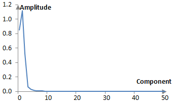
The fact that the discrete Fourier transform is computed with a small set of components – the length of the filter – means that the magnitude response would be sparse in the frequency domain, as shown on the following figure. Suppose that we take the sampling frequency of fs = 2000 Hz and we create a standard finite impulse response low pass filter with length N = 101 and cutoff frequency of fc = 40 Hz. The magnitude response of the filter in the figure below employs a transform of N = 101 points, which is the same as the length of the filter. The cutoff frequency is between components 2 and 3, which, given the sampling frequency of fs = 2000 Hz, translates to between 39.6 Hz and 59.4 Hz (sampling 101 times over 2000 Hz implies 19.8 Hz per component). Note that this figure is limited to component 50, or half of N.
With the discrete Fourier transform we can also compute the phase response of our low pass filter prototype. We note that the filter has coefficients that are symmetric around the middle, i.e., a(k) = a(N – 1 – K). Assume for a moment, that Re(H(n)) > 0. Then
$$\Phi_n=\mathrm{atan2}(Im(H(n)),Re(H(n)))=\mathrm{atan}(\frac{Im(H(n))}{Re(H(n))})$$ $$=\mathrm{atan}(\frac{\sum_{n=0}^{N-1} a(k) \, \sin(\frac{2\pi\,n\,k}{N})}{\sum_{n=0}^{N-1} a(k) \, \cos(\frac{2\pi\,n\,k}{N})})$$
Since a(k) = a(N – 1 – k),
$$a(k) \, \sin(\frac{2\pi\,k\,n}{N})+a(N-1-k) \, \sin(\frac{2\pi\,(N-1-k)\,n}{N})$$ $$=2 \, a(k) \, \sin(\frac{2\pi\,(N-1)\,n}{2N}) \, \cos(\frac{2\pi\,(N-1-2k)\,n}{2N})$$ $$a(k) \, \cos(\frac{2\pi\,k\,n}{N})+a(N-1-k) \, \cos(\frac{2\pi\,(N-1-k)\,n}{N})$$ $$=2 \, a(k) \, \cos(\frac{2\pi\,(N-1)\,n}{2N}) \, \cos(\frac{2\pi\,(N-1-2k)\,n}{2N})$$
The phase response, assuming that the filter is of odd length, is as follows.
$$\Phi_n=\mathrm{atan}(\frac{2 \, \sin(\frac{2\pi\,n}{N} \frac{N-1}{2}) (1+\sum_{k=0}^{(N-1)/2} (a(k) \cos(\frac{2\pi\,n}{N} \frac{N-1-2k}{2})) )}{2 \, \cos(\frac{2\pi\,n}{N} \frac{N-1}{2}) (1+\sum_{k=0}^{(N-1)/2} (a(k) \cos(\frac{2\pi\,n}{N} \frac{N-1-2k}{2})) )})$$
The "1 +" in the numerator and denominator handle the case when the filter is of odd length N. If the filter has even number of points N, the computations would be the same but without "1 +". Thus,
$$\Phi_n=\mathrm{atan}(\frac{\sin(\frac{2\pi\,n}{N} \frac{N-1}{2})}{\cos(\frac{2\pi\,n}{N} \frac{N-1}{2}) })=\frac{2\pi\,n}{N} \frac{N-1}{2}$$
The phase response of a finite impulse response filter with coefficients that are symmetric around the middle is linear with respect to the frequency n and produces a delay of (N – 1) / 2 samples. These computations assume that Re(H(n)) > 0, but are similar in other cases.
Using the inverse discrete Fourier transform
If the discrete Fourier transform produces the magnitude response of a filter, then we should be able to produce a filter by taking the inverse discrete Fourier transform from a desired magnitude response. The topic Low pass filter shows how to create a low pass filter by summing up the simple waves up to the cutoff frequency.
$$a(k)=\frac{2}{f_s} \sum_{n=1}^{f_c} \cos(\frac{2\pi\,n\,k}{f_s}), \, k=0,1,...,f_s-1$$
where fc is the cutoff frequency and fs is the sampling frequency. This equation can also be written as
$$a(k)=2(\frac{1}{f_s} \sum_{n=1}^{f_s / 2} B_n \, \cos(\frac{2\pi\,n\,k}{f_s})), \, B_n=\begin{cases} 1, n \le f_c \\ 0, n \gt f_c\end{cases}$$
where Bn is the desired magnitude response of the filter, equal to 1 up to the cutoff frequency fc and zero afterwards. The upper limit of the sum is fs / 2 as suggested by the Nyquist-Shannon sampling theorem.
This formula is very similar to the inverse discrete Fourier transform, except that it only takes the real part of the inverse discrete Fourier transform, hence only the cosines, is limited to half of the inverse transform, hence the sum goes up to only fs / 2, and is scaled by 2. Thus, this formula samples the frequency content and uses computations similar to the inverse discrete Fourier transform to create a filter. We are not limited to sampling only at fs, and we can sample at any evenly spaced N points. In other words, the low pass filter can be created by
$$a(k)=2(\frac{1}{N} \sum_{n=1}^{N / 2} B_n \, \cos(\frac{2\pi\,n\,k}{N})), \, B_n=\begin{cases} 1, \frac{n\,f_s}{N} \le f_c \\ 0, \frac{n\,f_s}{N} \gt f_c\end{cases} , \, k=0,1,...,N-1$$
We note that cosine functions are symmetric around the origin and that the filter a(k) could similarly be symmetric around the origin, if we are after a linear phase response. We can then extend the sum and remove the scaling factor of 2 as follows.
$$a(k)=\frac{1}{N} \sum_{n=-N/2}^{N / 2} B_n \, \cos(\frac{2\pi\,n\,k}{N}), \, B_n=\begin{cases} 1, |\frac{n\,f_s}{N}| \le f_c \\ 0, |\frac{n\,f_s}{N}| \gt f_c\end{cases}$$
Note the natural addition of n = 0 to the sum. Since Bn represents the desired filter magnitude response, the magnitude response should remain at 1 as the frequency approaches zero.
Finally, in an attempt to make the filter symmetric around (N – 1) / 2, we shift the filter as follows.
$$a(k)=\frac{1}{N} \sum_{n=-N/2}^{N / 2} B_n \, \cos(\frac{2\pi\,n\,(k-\frac{N-1}{2})}{N}), \, B_n=\begin{cases} 1, |\frac{n\,f_s}{N}| \le f_c \\ 0, |\frac{n\,f_s}{N}| \gt f_c\end{cases}, \, k=0,1,...,N-1$$
This filter formula resembles the inverse discrete Fourier transform, but it is not the inverse discrete Fourier transform. We do not use the inverse discrete Fourier transform to produce a FIR filter. There are important differences between the inverse transform and the filter computation above. First, the formula above uses only the real part of the inverse discrete Fourier transform. Second, the formula above is shifted both in n, as the sum runs from –N / 2 to N / 2 and in k, as the sum uses k – (N – 1) / 2.
The formula above is the real portion of a generalized or shifted form of the inverse complex valued discrete Fourier transform, which is usually written as
$$x(k)=\frac{1}{N} \sum_{k=0}^{N-1} H(n) \, e^{\frac{2\pi\,j\,(k+\alpha)\,(n+\beta)}{N}}$$
Note that we could easily add the imaginary part of the inverse discrete Fourier transform above. Since sine functions are odd (i.e., sin(-x) = -sin(x)), the sum of the sine values for n = -N / 2, …, N / 2 would simply be zero. In other words, by designing a desired magnitude response Bn that is symmetric around the origin, we created an inverse transform and thus a filter that contains only real valued coefficients.
Using a desired magnitude response that includes negative frequencies may be troublesome, since negative frequencies do not mean much. The technique of using a symmetric magnitude response to produce a real valued filter is, however, common.
Sampling of the continuous inverse Fourier transform
The continuous-time Fourier transform translates a signal x(t) that is a function of time for specific amplitudes, frequencies, and phase amounts into a signal H(x(t)) that is a function of frequencies and phase amounts for specific amplitudes and time. The inverse Fourier transform translates functions of frequencies and phase amounts into signals in time. An example of how the continuous inverse Fourier transform can be sampled to produce a low pass filter is shown in the topic Low pass filter.
Relationships between the Fourier transform and other transforms
The discrete-time Fourier transform is a special case of the Z transform. It is the Z transform evaluated at z = ejω = ej 2πf.
The continuous Fourier transform is equivalent to evaluating the bilateral Laplace transform with s = j ω = j 2πf.
Properties of the Fourier transform
The following are some of the more basic properties of the Fourier transform. Denote the Fourier transform of x(t) as in the definition above with Hs. Given integrable functions x(t) and y(t), complex numbers a and b, real numbers T and S, and the nonzero real number c
$$H(a\,x(t)+b\,y(t))=a\,H(x(t))+b\,H(y(t))$$ $$H(x(t-T))=e^{-j\,2\pi\,T\,s} H_s$$ $$H(e^{j\,2\pi\,t\,S}x(t)) = H_{s-S}$$ $$H(x(c\,t)) = \frac{1}{|c|} H_{s/c}$$ $$H(\overline{x(t)}) = \overline{H_{-s}}$$ $$H((x*y)(t)) = H(x(t)) \, H(y(t))$$
The first property is obviously the linearity of the Fourier transform. The second and third equations above are called the time shifting (or translation) properties. The fourth property shows scaling in the time domain. The fifth equation shows complex conjugation properties (this property explains the redundancy of the transform when used on real data). The last equation shows the transform of a convolution, which is useful when creating transfer functions of digital filters stacked one after the other.
A note on the fast Fourier transform
Using the discrete Fourier transform is quite computationally intensive. Each discrete Fourier transform of length N requires N2 multiplications of complex numbers. The fact that the number of computations in the discrete Fourier transform is proportional to N2 labels the transform as an O(N2) algorithm.
An alternative is to use the fast Fourier transform, or FFT. The FFT is not a transform, but is rather an algorithm for faster discrete Fourier transform computations. There are a number of good programmatic implementations of the FFT readily available and hence we will not present one here. We only present the theoretical foundation of the FFT, which is quite simple.
The FFT relies on the following equation, known as the Danielson-Lanczos lemma. The discrete Fourier transform of N points HN(x(k)), can be written as follows
$$H(n) = \sum_{k=0}^{N-1} x(k) \, e^{-\frac{2\pi\,j\,k\,n}{N}}$$ $$=\sum_{k=0}^{\frac{N}{2}-1} x(2k) \, e^{-\frac{2\pi\,2\,k\,n}{N}} + \sum_{k=0}^{\frac{N}{2}-1} x(2k+1) \, e^{-\frac{2\pi\,n\,(2k+1)}{N}}$$ $$=\sum_{k=0}^{\frac{N}{2}-1} x(2k) \, e^{-\frac{2\pi\,k\,n}{N/2}} + e^{-\frac{2\pi\,n}{N}} \sum_{k=0}^{\frac{N}{2}-1} x(2k+1) \, e^{-\frac{2\pi\,k\,n}{N/2}}$$ $$=H_{N/2}^{even}(x(k))+ e^{-\frac{2\pi\,k\,n}{N/2}} H_{N/2}^{odd} (x(k))$$
In other words, the discrete Fourier transform of N points can be computed as the sum of two discrete Fourier transforms of N / 2 points, where the first transform traverses the even points of the original discrete Fourier transform and the second transform traverses the odd points of the original transform. The second transform – of odd points – must be multiplied by some constant.
If we can split the discrete Fourier transform in to two transforms of length N / 2, then we can also split these two new transforms into four transforms of length N / 4. In fact, if we select the easy case where N is a power of 2, we can continue splitting up the transform into smaller transforms until we have a number of transforms of length 1.
For a discrete Fourier transform of length N, the FFT would require N transforms of length one and N complex computations because of the constants that appear in front of the transforms of the odd points. The FFT, however, would also require log2(N) operations to perform the discrete Fourier transform split into smaller transforms. Thus, the number of operations in the FFT is proportional to N log2(N), which means that the FFT is an O(N log2(N)) algorithm. On large sets of data, the FFT would be much faster than the discrete Fourier transform. For example, the discrete Fourier transform and FFT are useful in audio pitch shifting. A three-minute audio track may require up to 8 billion computations to be pitch shifted with the discrete Fourier transform, but it would require only about 80 million computations to be pitch shifted with the FFT.
Add new comment