Daubechies Daub4 wavelet transform

The level 1 Daubechies Daub4 wavelet transform of the signal x(k) of length N is x → (b₁ | a₁), where a₁ and b₁ are vectors of length N/2, computed from x via the inner products

$$a_1=(A_1*x,A_2*x,...,A_{N/2}*x)$$ $$b_1=(B_1*x,B_2*x,...,B_{N/2}*x)$$

with the vectors of length N

$$A_1=(\frac{1+\sqrt{3}}{4\sqrt{2}},\frac{3+\sqrt{3}}{4\sqrt{2}},\frac{3-\sqrt{3}}{4\sqrt{2}},\frac{1-\sqrt{3}}{4\sqrt{2}},0,0,0,0,...,0,0,0,0,0)$$ $$A_2=(0,0,\frac{1+\sqrt{3}}{4\sqrt{2}},\frac{3+\sqrt{3}}{4\sqrt{2}},\frac{3-\sqrt{3}}{4\sqrt{2}},\frac{1-\sqrt{3}}{4\sqrt{2}},0,0,...,0,0,0,0,0)$$ $$A_3=(0,0,0,0,\frac{1+\sqrt{3}}{4\sqrt{2}},\frac{3+\sqrt{3}}{4\sqrt{2}},\frac{3-\sqrt{3}}{4\sqrt{2}},\frac{1-\sqrt{3}}{4\sqrt{2}},...,0,0,0,0,0)$$ $$...$$ $$A_{\frac{N}{2}-1}=(0,0,0,0,0,0,0,0,...,\frac{1+\sqrt{3}}{4\sqrt{2}},\frac{3+\sqrt{3}}{4\sqrt{2}},\frac{3-\sqrt{3}}{4\sqrt{2}},\frac{1-\sqrt{3}}{4\sqrt{2}})$$ $$A_{\frac{N}{2}}=(\frac{3-\sqrt{3}}{4\sqrt{2}},\frac{1-\sqrt{3}}{4\sqrt{2}},0,0,0,0,0,0,...,0,0,\frac{1+\sqrt{3}}{4\sqrt{2}},\frac{3+\sqrt{3}}{4\sqrt{2}})$$

and

$$B_1=(\frac{1-\sqrt{3}}{4\sqrt{2}},\frac{-3+\sqrt{3}}{4\sqrt{2}},\frac{3+\sqrt{3}}{4\sqrt{2}},\frac{-1-\sqrt{3}}{4\sqrt{2}},0,0,0,0,...,0,0,0,0,0)$$ $$B_2=(0,0,\frac{1-\sqrt{3}}{4\sqrt{2}},\frac{-3+\sqrt{3}}{4\sqrt{2}},\frac{3+\sqrt{3}}{4\sqrt{2}},\frac{-1-\sqrt{3}}{4\sqrt{2}},0,0,...,0,0,0,0,0)$$ $$B_3=(0,0,0,0,\frac{1-\sqrt{3}}{4\sqrt{2}},\frac{-3+\sqrt{3}}{4\sqrt{2}},\frac{3+\sqrt{3}}{4\sqrt{2}},\frac{-1-\sqrt{3}}{4\sqrt{2}},...,0,0,0,0,0)$$ $$...$$ $$B_{\frac{N}{2}-1}=(0,0,0,0,0,0,0,0,...,\frac{1-\sqrt{3}}{4\sqrt{2}},\frac{-3+\sqrt{3}}{4\sqrt{2}},\frac{3+\sqrt{3}}{4\sqrt{2}},\frac{-1-\sqrt{3}}{4\sqrt{2}})$$ $$B_{\frac{N}{2}}=(\frac{3+\sqrt{3}}{4\sqrt{2}},\frac{-1-\sqrt{3}}{4\sqrt{2}},0,0,0,0,0,0,...,0,0,\frac{1-\sqrt{3}}{4\sqrt{2}},\frac{-3+\sqrt{3}}{4\sqrt{2}})$$

The level 2 Daubechies Daub4 wavelet transform is x → (b₁ | b₂ | a₂), where a₂ and b₂ are the level 1 Daubechies Daub4 wavelet transform of a₁, computed with vectors A and B of length N / 2. The level N Daubechies Daub4 wavelet transform is computed by successively taking the transforms of the "a" portion of the previous level of the transform, with vectors that are of length equal to half of the length of the previous transform.

Note that x(k) can be reconstructed from a₁ and b₁ with the computation

$$x(k)=\sum_{i=0}^{N-1}A_i(k)a_1(i)+\sum_{i=0}^{N-1}B_i(k)b_1(i)$$

In the level 2 transform, a1 can be reconstructed from a₂ and b₂ and thus x(k) can be reconstructed from b₁, b₂, and a₂ (hence, a₁ is omitted from the definition of the transform x → (b₁ | b₂ | a₂)).

In each successive iteration, the "a" and "b" vectors are of length equal to half of the length of the previous level transform. Thus, if N = 2ⁿ for some integer n, we can write x → (b₁ | b₂ | … | b_N-1 | a_N-1), where a_N-1 and b_N-1 are vectors of length 2 (unlike when using the Haar wavelet transform, we cannot get to level N and vectors a_N and b_N of length 1, as the A and B vectors have four nonzero values rather than just two). Note that b₁ is of length N / 2, b₂ is of length N / 4 and so on. The combined length of b₁, b₂, …, b_N-1, a_N-1 is N and so these vectors carry the same amount of information as x(k). Since x(k) can be reconstructed from these vectors, they carry the same information as x(k).

As in the Haar wavelet transform, a₁ averages the signal x(k) and is the "trend" of the signal. b₁ contains the fluctuations that a₁ removes. a₁ is computed as the convolution of the signal x(k) with A₁ (with the caveat that the step of this convolution is two samples, rather than one). b₁ is the convolution of the signal x(k) with B₁. In other words, a₁ and b₁ are the results of a low pass filter and a high pass filter on x(k) (the vectors A₁ and B₁). Similarly, a₂ and b₂ are the trend and fluctuations of a₁ and so on.

The Daub4 wavelet transform is only one of the Daubechies wavelet transforms.

Data compression example with the Daubechies Daub4 wavelet transform

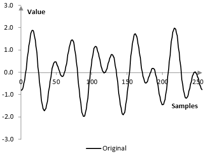
Take the signal x(k) of length N = 256 that consists of two simple waves with frequencies 5 Hz and 9 Hz, given the sampling frequency 256 Hz. The phase of the 9 Hz frequency is 10 samples and the phase of the 5 Hz frequency is zero. The signal is

$$x(k)=\sin(\frac{2\pi\,k\,5}{256})+\sin(\frac{2\pi\,(k-10)\,9}{256})$$

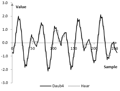
A detailed example of compressing this signal is provided in the topic Haar wavelet transform. This example here compares the results of the Haar and Daubechies Daub4 wavelet transforms.

Decompose this signal using the Daubechies Daub4 wavelet transform into b₁, b₂, …, b₇, and a₇. Sort all values of these vectors (as one single array) and remove the smallest values (replace them with 0). If we need to transmit the signal, we can transmit only the nonzero values. We can use bitmasks to denote where the nonzero values should be placed when the b₁, …, a₇ vectors are reconstructed and we can then reconstruct the signal x(k) from these vectors. This will result in transmitting less data, than the signal x(k) itself.

In the example described in the topic Haar wavelet transform, for example, removing half of all values (the smaller values) allowed the transform to retain 99.5% of the energy of the signal, where the energy is computed as the sum of the squares of the values of the transform. Since half of the values were zeroed out, the compression ratio in that example was 2:1. In the Daubechies Daub4 wavelet transform of this same signal, 99.5% of the energy can be retained if only a fifth of the values are retained and four fifths are zeroed out. That is, the same amount of energy can be retained with 5:1 compression. If 5:1 compression is used in the Haar wavelet transform, the loss of energy will be over 5%, which is significant.

The reconstructed signal x(k), after a number of values are removed from the vectors b₁, …, a₇, is not the same as the original, of course. The following graphs show the two signals.

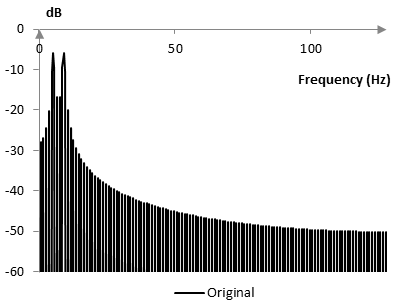
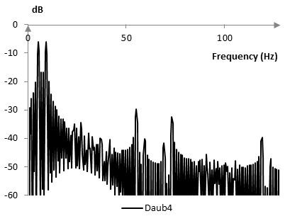
The frequency content of the reconstructed signal is also different. The following two graphs show a zoom in the Fourier transform of the original and reconstructed signals.