Square wave

A square wave is a periodic function that takes only two values – a minimum and a maximum – and alternates between these two values in equal intervals.

In discrete time, for example, if N is the period of the function, then the function

$$x(k)=\begin{cases} -1, \,\, k \mod \, N \lt\frac{N}{2} \\ 1, \,\, k \mod N \ge \frac{N}{2} \end{cases}$$

is a square wave. It alternates between -1 and 1. Its period is N samples. It takes each value for an interval equal to N/2 samples before switching to the other value.

Alternatively,

$$x(k)=\mathrm{sgn}(\sin(\frac{2 \pi\,k\,f}{f_s}))$$

since the sign function "sgn" is equal to 1 when its argument is positive and to -1 when its argument is negative. However, care must be taken where the argument is zero, as, as usually defined, sgn(0) = 0. Here, f is the desired square wave frequency and f_s is the sampling frequency.

If, for example, N = 60, then the first function above will be as follows.

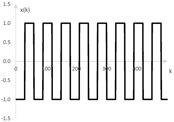
The following is a square wave with the frequency of middle C.

Click Play to hear a square wave.

Using square waves

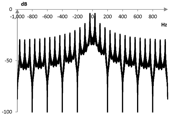
Analysis of the frequency content of square waves show that they can be thought of as the combination of many harmonics. Below, for example, is the discrete Fourier transform of 500 components of the example square wave above.

The harmonics in the square wave are all integer multiples of the frequency of the square wave. Note the evenly occurring notches in the magnitudes of frequencies present in the square wave.

Because of these harmonics, square waves are often used in synthesizers. Square waves with the desired harmonics can be combined and the result filtered (e.g., through a low pass filter) to synthesize a sound resembling the sound of a specific instrument.

Harmonics of the square wave

The peaks in the Fourier transform of a square wave with frequency f occur at all odd harmonics of f, which are (2k – 1) f, k = 1, 2, …. For example, since the frequency of the square wave in the graph above is 33.3 Hz, the peaks occur at 33.3 Hz, 100 Hz, 166.7 Hz, 233.3 Hz, and so on.

In other words, the Fourier series expansion of the square wave is an infinite series of the odd harmonics of the square wave frequency.

Fourier series expansion of the square wave

The Fourier series expansion at sample k of the square wave is as follows.

$$\frac{4}{\pi} \sum_{n=1}^\infty \frac{\sin(\frac{2\,\pi\,k\,(2n-1)\,f}{f_s})}{2\,n -1}$$

where f is the frequency of the square wave and f_s is the sampling rate.

The following four graphs show the first term of the series sum, the sum of the first two terms, the sum of the first three terms, and the sum of the first eight terms for f = 33.3 Hz, f_s = 16000 Hz and for the first 500 or so samples k on the horizontal axis.

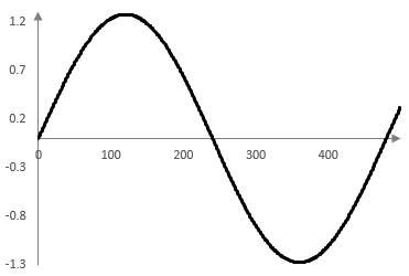
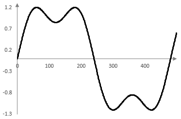
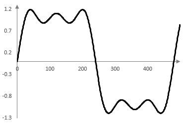
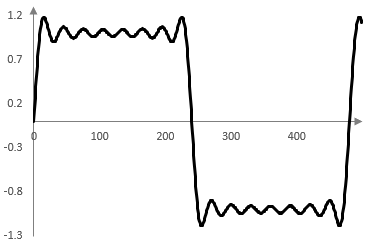
The ripples at the points where the square wave changes value are the result of the Gibbs phenomenon – approximating a discontinuous function with a continuous function.