In mathematics, the Gibbs phenomenon appears whenever the Fourier series – a series of continuous functions – is used to approximate a discontinuous continuously differentiable function. At the points of discontinuity, the partial Fourier series, rather than approximating precisely the discontinuous function, shows ripples. These ripples typically increase in number and frequency as the approximation improves, decrease in energy / RMS amplitude, and do not die out but settle to a fixed height.
In digital signal processing, since the desired magnitude response of finite impulse response filters is usually a discontinuous function, the actual magnitude response of the filters produces ripples at the point of discontinuity, which increase in number and frequency as the length of the filter increases, decrease in RMS amplitude, but do not die out and settle to a fixed height of, as shown below, approximately 0.08949 normalized amplitude. These ripples are a manifestation of the Gibbs phenomenon.
Manifestation of the Gibbs phenomenon with finite impulse response filters
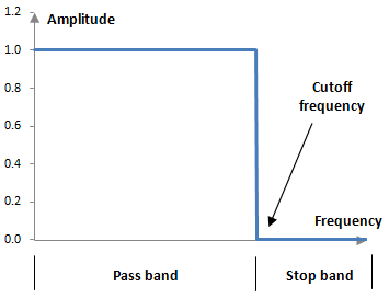
The desired magnitude response of a low pass filter is discontinuous, as an ideal magnitude response over the frequency spectrum should return a normalized amplitude of 1 (the original amplitude of the signal) up to the cutoff frequency and an amplitude of 0 afterwards. The following is the magnitude response of an ideal low pass filter.
The following picture shows the typical magnitude response of a digital finite impulse response low pass filter.
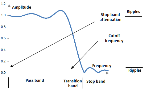
The magnitude response of a typical finite impulse response low pass filter is in fact a Fourier series approximation of the desired magnitude response. Two derivations of the formulae for such low pass filters are shown in the topic Low pass filter. The ripples in the pass band and in the stop band in the actual magnitude response above are a manifestation of the Gibbs phenomenon.
The following picture compares the magnitude responses in the pass band of three low pass filters with lengths of 100 points, 200 points, and 300 points. All three filters have a cutoff frequency of 40 Hz. The sampling frequency is 2000 Hz.
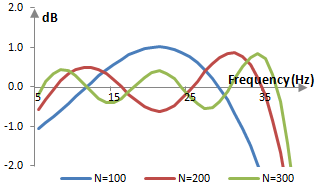
A filter of larger length, the magnitude response of which is a better approximation to the desired ideal magnitude response, produces more but smaller ripples (with less energy). As the length of the filter increases, the ripples do not disappear, but settle on a final height.
An example Gibbs phenomenon in an equalizer
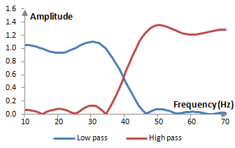
An interesting manifestation of Gibbs phenomenon can be seen when designing equalizers based on finite impulse response filters. The following figure shows the magnitude responses of two filters – one low pass and one high pass – with the same cutoff frequency of 40 Hz over the sampling rate of 2000 Hz. A gain of 2 dB has been added to the high pass filter.
When the filters are combined and their coefficients are added, they produce an equalizer that adds 2 dB to frequencies above 40 Hz. The magnitude response of the equalizer is as follows.
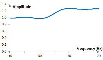
Note that the ripples of the equalizer are smaller than the ripples of each individual filter. As we will show below, the amount by which the Gibbs phenomenon ripple overshoots the desired magnitude response is proportional to the jump at the discontinuity (with a factor of approximately 1.089494). Since the discontinuity of the magnitude response of the equalizer is smaller (2 dB, from normalized amplitude of 1 to normalized amplitude of 1.259) than the discontinuity of the low pass filter or the high pass filter (from normalized amplitude of 0 to normalized amplitude of 1), the ripples are smaller.
Quantifying the Gibbs phenomenon
A finite impulse response filter a(k) of length N computes the values of the output signal y(k) from the values of the input signal x(k) with the formula
$$y(k)=\sum_{n=0}^{N-1} a(n) \, x(k-n)$$
The Z transform of the output of a finite impulse response filter is as follows.
$$Z(y(k))=Z(\sum_{n=0}^{N-1} a(n) \, x(k-n))=Z(x(k)) \sum_{n=0}^{N-1} a(n) \, z^{-n}$$
The general transfer function of a finite impulse response filter then is
$$H(z)=\sum_{k=0}^{N-1} a(k) \, z^{-k}$$
A typical finite impulse response filter is designed to have coefficients that are symmetric around the middle, as that ensures a linear phase response and a filter with real valued coefficients. We can combine the first and last term, the second and second last term, and so on, and we can denote M = (N – 1) / 2. At the unit circle, at z = e-j ω
$$a(k) \, z^{-k} + a(N-1-k) \, z^{k-(N-1)}$$ $$=z^{-M} \, a(k) \, (z^{M-k}+z^{k-M})$$ $$=2 z^{-M} \, a(k) \, \cos(\omega (k-M))$$
and the magnitude response, given the transfer function above, becomes
$$|H(e^{-j\,\omega})|=|z^{-M}(a(M)+2\sum_{k=0}^{M-1} a(k) \, \cos(\omega(k-M)))|$$ $$=a(M)+ 2\sum_{k=0}^{M-1} a(k) \, \cos(\omega(k-M))$$
This is a real valued continuous function. It allows us to illustrate the Gibbs phenomenon. Rewrite the magnitude response, using the definition of a(k) from the low pass filter formula
$$a(k)=\begin{cases} \frac{\sin(\frac{2\pi\,f_c\,(k-\frac{N-1}{2})}{f_s})}{\pi(k-\frac{N-1}{2})}, k \ne \frac{N-1}{2} \\ 2\frac{f_c}{f_s}, k = \frac{N-1}{2} \end{cases}$$
where the cutoff frequency is ωc = 2 π fc / fs, and substitute n = k – M.
$$|H(e^{-j\,\omega})|=a(M) + 2 \sum_{k=0}^{M-1} \frac{\sin(\omega_c (k-M)) \, \cos(\omega (k-M))}{\pi(k-M)}$$ $$=a(M) + 2 \sum_{n=1}^{M} \frac{\sin(\omega_c\,n) \, \cos(\omega\,n)}{\pi\,n}$$ $$=a(M) + \frac{\omega_c+\omega}{\pi} \sum_{n=1}^{M} \frac{\sin((\omega_c+\omega)n)}{(\omega_c+\omega)n}+ \frac{\omega_c-\omega}{\pi} \sum_{n=1}^{M} \frac{\sin((\omega_c-\omega)n)}{(\omega_c-\omega)n}$$
Now set ω = ωc + π / M. The second sum above becomes
$$\frac{1}{M} \sum_{n=1}^{M} \frac{\sin(\frac{\pi\,n}{M})}{\frac{\pi\,n}{M}}$$
As M approaches infinity and ω approaches ωc from the right, the sum approaches the known integral between 0 and 1 of the sinc function
$$\int_{0}^{1} \frac{\sin(\pi\,t)}{\pi\,t} \approx \frac{1}{2} + 0.08949$$
and thus
$$\lim_{\omega \rightarrow \omega_c+} |H(e^{-j\,\omega})|=a(M)+\frac{2\omega_c}{\pi} \sum_{n=0}^{M} \frac{\sin(2\omega_c\,n)}{2\omega_c\,n}-\frac{1}{2}-0.08949$$
Now set ω = ωc – π / M. The same second sum above is
$$-\frac{1}{M} \sum_{n=1}^{M} \frac{\sin(-\frac{\pi\,n}{M})}{-\frac{\pi\,n}{M}}$$
As M approaches infinity and this time ω approaches ωc from the left, the sum approaches
$$-\int_{0}^{1} \frac{\sin(\pi\,t)}{\pi\,t} \approx -(\frac{1}{2}+0.08949)$$
and thus
$$\lim_{\omega \rightarrow \omega_c-} |H(e^{-j\,\omega})|=a(M)+\frac{2\omega_c}{\pi} \sum_{n=0}^{M} \frac{\sin(2\omega_c\,n)}{2\omega_c\,n}+\frac{1}{2}+0.08949$$
The two limits differ by approximately 1.17898. The desired magnitude response, on the other hand, has a jump at the point of discontinuity of only 1. This is an illustration the Gibbs phenomenon.
Position of the ripples
This does not mean that the Gibbs phenomenon ripples occur at ω = ωc +/- π / M. If we wanted to find the ripple, the maximum of the magnitude response |H(e-j ω)|, we would presumably start by taking the derivative of that magnitude response. With the representation above, the derivative of the magnitude response would consist of two series of cosines, which can be summed up with the Dirichlet kernel. However, the resulting derivative would probably still be too complex to work with. The easiest thing to do is to solve for the maximum numerically – programmatically.
The figure below shows the normalized angular frequency ω at which the maximum the magnitude response occurs for filters at different lengths N.
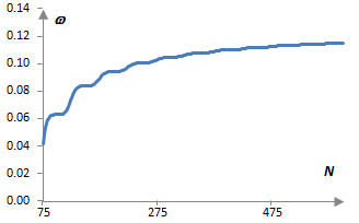
These are low pass filters with cutoff frequency fc = 40 Hz at the sampling frequency fs = 2000 Hz. As the length of the filter increases, ω approaches the normalized cutoff frequency ωc = 2π fc / fs = 0.126. The step-wise behavior of the plot is due to the fact that we are working only with integer N. Values for N < 75 are not shown as such filters do not have ripples. Their magnitude response starts below 1 and continues down with higher frequencies.
Reducing the Gibbs phenomenon ripples
The Gibbs phenomenon ripples can be reduced by windowing finite impulse response filters. For example, one can use a Blackman window, Hann window, Hamming window, Tukey window, Gaussian window, Kaiser window, and many others. Windowing, although reducing the ripples and usually improving the stop band attenuation of the filter, comes at the expense of wider transition bands.
Add new comment