The Laplace transform is defined by
$$\mathcal{L}(f(t))=\int_0^{\infty} f(t)\,e^{-st}\,dt$$
where s = σ + j ω, for the angular frequency ω and the scalar σ. The inverse Laplace transform is given by
$$f(t)=\frac{1}{2\pi i}\lim_{t \rightarrow \infty} \int_{\gamma - iT}^{\gamma+iT}e^{st} \mathcal{L}(f(t)) ds$$
where γ is a real number necessary for the convergence of L(f(t)).
Relationship between the Laplace transform, the Z transform, and Fourier transforms
Although the Laplace transform is a transform of continuous-time functions, whereas the Z transform is a transform of discrete-time functions, the computations of the two are similar. This said, rather than producing a function of the variable
$$z=A\,e^{-j \omega}$$
the Laplace transform produces a function of the variable
$$s=\sigma+j \, \omega$$
Mathematically, when a continuous signal is sampled, it is convolved with an infinite series of impulses called a Dirac comb (an infinite series of Dirac delta functions (impulses), which have an integral of one from negative infinity to infinity). Thus, if a discrete signal x(k), sampled at the sampling time T = 1 / fs, where fs is the sampling frequency, has a continuous representation x(t), then its Laplace transform is
$$\int_0^\infty x(t) e^{-st}dt=\int_0^\infty (\sum_{k=0}^\infty x(k)\delta(t-kT)e^{-st}) dt$$ $$\sum_{k=0}^\infty (x(k) \int_0^\infty \delta(t-kT)e^{-st}dt)=\sum_{k=0}^\infty x(k) e^{-ksT}$$
Thus, the Laplace transform of a sampled signal is the unilateral Z transform, with z = esT. This means that the Laplace transform is also related to the discrete-time Fourier transform, which is a special case of the Z transform (the Z transform with A = 1). The Laplace transform is also related to the continuous Fourier transform, which is simply the Laplace transform with σ = 0.
Motivation for using the Laplace transform in digital signal processing
Just like the Fourier transform and the Z transform, we can think of the Laplace transform in digital signal processing as translating a function of time given specific amplitudes, frequencies, and phase amounts into a function of frequencies and phase amounts for specific amplitudes and time. Just as we typically use the Z transform in digital signal processing on the unit circle (with A = 1 and z = e-j ω), we typically use the Laplace transform with σ = 0 and s = j ω. The motivation for using the Laplace transform, as opposed to the Z transform, in digital signal processing is simple. Transfer functions produced by the Laplace transform and expressed as functions s = j ω are much simpler functions of the angular frequency ω than transfer functions produces with the Fourier transform or the Z transform.
It is easy, for example, to take the desired magnitude response of the Butterworth low pass filter
$$|H(j\omega)|=\frac{G}{\sqrt{1+(\frac{\omega}{\omega_c})^{2n}}}=\frac{G}{\sqrt{1+(\frac{\omega^2}{\omega_c^2})^{n}}}$$
and see that the squared transfer function, with s = j ω, should be something like
$$H(s)^2=\frac{G^2}{1+(\frac{-s^2}{\omega_c^2})^{n}}=\frac{G^2}{1+(\frac{-s}{\omega_c})^{2n}}$$
(Usually, rather than writing H(s)2, we will write H(s)H(-s). These types of transforms produce redundant information on real data and, since we want to produce a filter with real-valued coefficients, we can assume that the magnitude response is symmetric around the origin and that H(s) = H(-s).) We can then solve for the roots of the denominator
$$1+(\frac{-s}{\omega_c})^{2n}=0$$ $$s_k=\pm \omega_c e^{\frac{j(2k-1)\pi}{2n}}, k=1,2,...,2n$$
and derive
$$H(s)^2=G^2 \prod_{k=1}^{2n} \frac{1}{s-s_k}$$
We know that a stable system is one that produces reasonable (bound) response to any reasonable (bound) input. The Laplace transform of such system must be bound. Since in practice we only work with nonnegative amplitudes, we want a Laplace transform transfer function be bound for all s for which σ = Re(s) ≥ 0. If the transfer function has denominator roots (poles) where it is not bound, these roots must have negative real parts.
We can now clearly define the transfer function of the Butterworth low pass filter.
$$H(s)=\frac{G\,\omega_c^n}{\prod_{k=1}^n (s-s_k)}, s_k=\omega_c \, e^{\frac{j(2k+n-1)\pi}{2n}}$$
The derivation of the Butterworth low pass filter would be much more difficult with the Z transform.
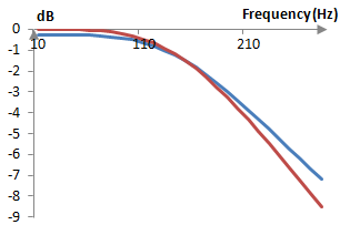
A disadvantage of the Laplace transform is that such continuous-time descriptions of digital signal processing systems must be converted into discrete-time descriptions – usually to the Z transform. One way to do so is to use the inverse Laplace transform. Another way to do so is to use the bilinear transformation. Both methods are shown in the topic Butterworth filter. The bilinear transformation filter performs better and is easier to derive. The bilinear transformation, however, warps the frequency domain. A digital Butterworth filter with a cutoff frequency ωa, before the bilinear transformation will have a cutoff frequency of ωd = 2 arctan(ωa / 2) after the bilinear transformation. When designing filters, we must be careful to pick the right cutoff frequency. This said, the bilinear transformation is an appropriate translation of the Laplace transform to the Z transform. The following graph shows the magnitude response of an example second order impulse invariant (using the inverse Laplace transform) Butterworth filter (blue) and the same filter computed with the bilinear transformation (red).
A second disadvantage is that the Laplace transform is that its notation is not as easy as the notation of the Z transform. For example, the time-shifting property of the Z transform is
$$\mathcal{Z}(x(k-m))=\mathcal{Z}(x(k))z^{-m}$$
The same time-shifting property of the Laplace transform is
$$\mathcal{L}(f(t-a)u(t-a))=\mathcal{L}(f(t))e^{-as}, u=\int_{-\infty}^x \delta(t)dt$$
where u(t) is the Heaviside step function and δ is the Dirac delta function.
Transfer functions using the Laplace transform
The Laplace transform transfer function of a continuous-time system with input signal x(t) and output signal y(t) would be
$$H(s)=\frac{\mathcal{L}(y(t))}{\mathcal{L}(x(t))}$$
As with the Z transform, we can use the Laplace transform to evaluate the magnitude and phase responses of the system, but we must do so on the unit circle, i.e., at σ = 0 and s = j ω. The magnitude response of a system with the transfer function above would be |H(j ω)| and its phase response is arg(H(j ω)).
Example Laplace transform transfer functions for various filters are given in the topics: Bessel filter , Butterworth filter, Chebychev filter (Type I) , Chebychev filter (Type II), Notch filter, Peak filter, and Shelving filter.
Add new comment