Butterworth filter

The Butterworth filter is given by the normalized transfer function

$$H(S)=\frac{1}{B_n(S)}$$

where n is the order of the filter and B_n(S) are the normalized Butterworth polynomials given by

$$B_n(S)=\prod_{k=1}^{\frac{n}{2}}(S^2-2\,\cos(\frac{2k+n-1}{2n}\pi)S+1)$$ $$B_n(S)=(S+1)\prod_{k=1}^{\frac{n-1}{2}}(S^2-2\,\cos(\frac{2k+n-1}{2n}\pi)S+1)$$

for n even and n odd respectively.

This transfer function is normalized (i.e., it is for the Butterworth low pass filter with cutoff frequency 1). Substituting S = s / ω_c produces the Laplace transform transfer function of the Butterworth low pass filter, where ω_c is the cutoff frequency of the filter. Substituting S = ω_c / s produces the Butterworth high pass filter. Substituting S = (s² + ω_c²) / (B s) produces the Butterworth band pass filter, where ω_c is the midpoint of the pass band and B is the width of the band. Substituting S = B s / (s² + ω_c²) produces the Butterworth band stop filter.

Example: transfer function of the second order low pass Butterworth filter

Substituting S = s / ω_c and n = 2 produces the transfer function

$$H(s)=\frac{1}{(\frac{s}{\omega_c})^2+\sqrt{2}(\frac{s}{\omega_c})+1}$$

In general, for any order n, the transfer function of the low pass Butterworth filter can also be written as

$$H(s)=\frac{\omega_c^n}{\prod_{k=1}^{n}(s-s_k)}, \, s_k=\omega_c\,e^{\frac{j(2k+n-1)\pi}{2n}}$$

To compute the specifications of either digital or analog Butterworth filters from this transfer functions, one must use a significant amount of algebraic / mathematical manipulations. Generally, there are two methods, examples of which are presented below. The first method uses inverse Laplace transforms. It is more mathematically involved, but does not warp the magnitude response of the analog filter. The second method uses the bilinear transformation. It is easier to implement and performs well for digital filters, although it is an approximation.

Example of an impulse invariant second order Butterworth low pass filter

Use the general form of the Butterworth low pass transfer function and set n = 2. The transfer function becomes

$$H(s)=\frac{\omega_c^2}{(s-s_1)(s-s_2)}$$

Using the definition of s_k and partial fraction expansion we get

$$H(s)=\frac{-j\frac{\omega_c}{2 \sin(\frac{3\pi}{4})}}{s-s_1}+\frac{j\frac{\omega_c}{2 \sin(\frac{3\pi}{4})}}{s-s_2}$$

The filter's impulse response can be obtained with the inverse Laplace transform. The continuous (analog) impulse response is

$$y(t)=(-j\frac{\omega_c}{2 \sin(\frac{3\pi}{4})}e^{s_1 t}+j\frac{\omega_c}{2 \sin(\frac{3\pi}{4})}e^{s_2 t}) \, x(t)$$

where y(t) is the output signal and x(t) is the input signal. Substitute t with k to get the discrete form of the impulse response. The Z transform of the impulse response then is

$$H(z)=\frac{j \frac{\omega_c}{2 \sin(\frac{3 \pi}{4})}}{1-e^{s_1}z^{-1}}-\frac{j \frac{\omega_c}{2 \sin(\frac{3 \pi}{4})}}{1-e^{s_2}z^{-1}}$$

Combine the two terms and use the fact that s₁ and s₂ are complex conjugates and that s₁ s₂ = ω_c² and s₁+ s₂ = 2 ω_c cos(3π/4).

$$H(z)=\frac{-\frac{\omega_c}{\sin(\frac{3 \pi}{4})} \sin(\frac{\omega_c}{\sin(\frac{3 \pi}{4})}) \,e^{\omega_c \, \cos(\frac{3 \pi}{4})} z^{-1}}{1-2 \cos(\frac{\omega_c}{\sin(\frac{3 \pi}{4})}) \, e^{\omega_c \, \cos(\frac{3 \pi}{4})} z^{-1}+e^{2 \omega_c \, \cos(\frac{3 \pi}{4})} z^{-2}}$$

The second order Butterworth low pass filter then is

$$y(k)=-\sqrt{2} \omega_c \, \sin(\frac{\omega_c}{\sqrt{2}}) \, e^{-\frac{\omega_c}{\sqrt{2}}} x(k-1)$$ $$+2 \,\cos(\frac{\omega_c}{\sqrt{2}}) \, e^{-\frac{\omega_c}{\sqrt{2}}} y(k-1)-e^{-\sqrt{2}\,\omega_c} y(k-2)$$

where y(k) is output signal and x(k) is input signal.

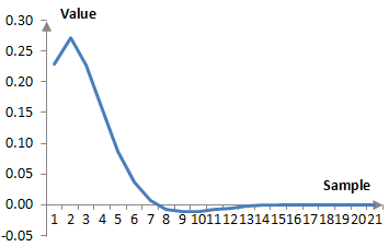
Suppose, for example, that the cutoff frequency is ω_c = 0.6. The transfer function becomes

$$H(z)=\frac{-0.22853 \, z^{-1}}{1-1.19249\,z^{-1}+0.42804\,z^{-2}}$$

and the filter itself is given by

$$y(k)=-0.22853 \, x(k-1)+1.19249\,y(k-1)-0.42804\,y(k-2)$$

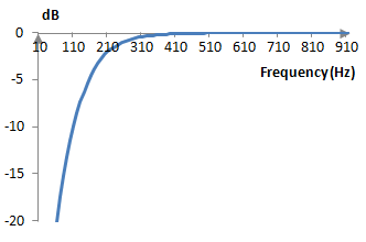
The following graph shows how the filter responds to an impulse.

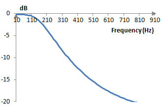
Given sampling frequency of, say, 2000 Hz, the cutoff frequency translates to ω_c = (0.6 * 2000 / (2π)) = 191 Hz. The magnitude response of this example filter is shown on the graph below.

Example of a second order Butterworth low pass filter using the bilinear transformation

An easier way to compute the Z transform transfer function for the Butterworth filter is to use bilinear transformation. The relationship between the Laplace transform and the Z transform is z = e^sT, where T is the sampling time (i.e., T = 1/ f_s, where f_s is the sampling frequency). Thus

$$s=\frac{1}{T}ln(z) \approx \frac{2}{T} \frac{z-1}{z+1}$$

Setting, as is usually assumed, T = 1 and substituting s = 2 (z – 1) / (z + 1), we get

$$H(z)=\frac{a_0+a_1 z^{-1}+a_2 z^{-2}}{b_0+b_1 z^{-1}+b_2 z^{-2}}$$ $$a_0=\omega_c^2$$ $$a_1=2\omega_c^2$$ $$a_2=\omega_c^2$$ $$b_0=4-4\omega_c \, \cos(\frac{3 \pi}{4})+\omega_c^2$$ $$b_1=-8+2\omega_c^2$$ $$b_2=4+4\omega_c \, \cos(\frac{3 \pi}{4})+\omega_c^2$$

Suppose again that the cutoff frequency is ω_c = 0.6 (technically, ω_c = 2 arctan(0.6/2) ≈ 0.583, because of the warping of the frequency domain by the bilinear transformation). After scaling to obtain 1 at the beginning of the denominator, we get

$$H(z)=\frac{0.059435+0.118870z^{-1}+0.059435z^{-2}}{1-1.201904z^{-1}+0.439643z^{-2}}$$

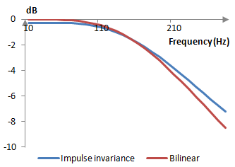
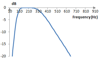
This filter is different than the impulse invariant filter described above, because the bilinear transformation is an approximation. Here are the magnitude responses of the two filters.

The bilinear transformation filter performs better and is easier to derive. The bilinear transformation, however, warps the frequency response of the filter. A digital Butterworth filter with a cutoff frequency ω_d, if implemented in the analog world, will have a cutoff frequency of ω_a = 2 tan(ω_d/2), and when designing analog filters, we must be careful to pick the right analog cutoff frequency. This said, the bilinear transformation is the easier and more commonly used method.

Higher order Butterworth filters

When designing higher order Butterworth filters we have two choices. We can use the methods above. Those are tedious, as there are a lot of computations involved. Alternatively, we can recognize that the roots s_k of the denominator of H(s) are complex conjugate pairs. For example, in a Butterworth filter of order 4, s₁ and s₄ are a pair and s₂ and s₃ are a pair.

$$s_1=\omega_c \, e^{j \frac{5 \pi}{8}}$$ $$s_2=\omega_c \, e^{j \frac{7 \pi}{8}}$$ $$s_3=\omega_c \, e^{j \frac{9 \pi}{8}}=\omega_c \, e^{-j \frac{7 \pi}{8}}$$ $$s_4=\omega_c \, e^{j \frac{11 \pi}{8}}=\omega_c \, e^{-j \frac{5 \pi}{8}}$$

We can rewrite H(s) for the fourth order low pass Butterworth filter as follows.

$$H(s)=(\frac{\omega_c^2}{(s-s_1)(s-s_4)})(\frac{\omega_c^2}{(s-s_2)(s-s_3)})$$

Both multiples above have real coefficients, since they use complex conjugates. The multiplication of the two transfer functions of two filters of order 2 means that the impulse response of the total filter is the convolution of the impulse responses of the two filters and the filters must be stacked one after the other. The output of the first filter will become the input to the second filter (these are not Butterworth filters, as the roots s_k are not the Butterworth ones for order 2, although the bilinear transformation computations use the same computations).

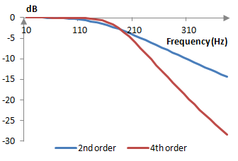
The following graph compares the magnitude responses of the second and fourth order Butterworth filters, where the fourth order Butterworth filter is implemented as two second order filters stacked one after the other and where both filters are computed using bilinear transformations. Note that the two filters cross at around -3 dB, which, typically of Butterworth filters, happens at the cutoff frequency. Here the sampling frequency again is 2000 Hz and the cutoff frequency is ω_c = (0.6 * 2000 / (2 π)) = 191 Hz.

Example of a second order high pass Butterworth filter

Substitute S = ω_c / s and n = 2 in the transfer function at the top of this topic to obtain

$$H(s)=\frac{1}{(\frac{\omega_c}{s})^2+\sqrt{2}(\frac{\omega_c}{s})+1}$$

This is the transfer function of the second order high pass Butterworth filter. Use the bilinear transformation s = 2 (z – 1) / (z + 1) to rewrite this transfer function as follows.

$$H(z)=\frac{4-8z^{-1}+4z^{-2}}{(\omega_c^2-2\sqrt{2}\omega_c+4)+(2\omega_c^2-8)z^{-1}+(\omega_c^2+2\sqrt{2}\omega_c+4)z^{-2}}$$

When ω_c = 0.6 for example, then the transfer function is

$$H(z)=\frac{0.6603-1.3208z^{-1}+0.6604z^{-2}}{1-1.2019z^{-1}+0.4396z^{-2}}$$

Take a sampling frequency of, say, 2000 Hz. The cutoff frequency translates to ω_c = 191 Hz, and the transfer function above produces a filter with the following magnitude response.

Example of a second order band pass Butterworth filter

Substitute S = (s² + ω_c²) / (B s) and n = 2 to obtain the second order Butterworth band pass filter. The Butterworth band pass and band stop filters take a lot of algebraic manipulation and it is probably easier to simply stack low pass and high pass filters. In any case, the transfer function of the second order Butterworth band pass filter after the bilinear transformation is as follows.

$$H(z)=\frac{a_0+a_2z^{-2}+a_4z^{-4}}{b_0+b_1z^{-1}+b_2z^{-2}+b_3z^{-3}+b_4z^{-4}}$$ $$a_0=4B^2$$ $$a_2=-8B^2$$ $$a_4=4B^2$$ $$b_0=16+8\sqrt{2}B+4(2\omega_c^2+B^2)+2\sqrt{2}B\omega_c^2+\omega_c^4$$ $$b_1=-64-16\sqrt{2}B+4\sqrt{2}B\omega_c^2+4\omega_c^4$$ $$b_2=96-8(2\omega_c^2+B^2)+6\omega_c^4$$ $$b_3=-64+16\sqrt{2}B-4\sqrt{2}B\omega_c^2+4\omega_c^4$$ $$b_4=16-8\sqrt{2}B+4(2\omega_c^2+B^2)-2\sqrt{2}B\omega_c^2+\omega_c^4$$

Using, for example, ω_c = 0.6 and B = 1 produces the filter

$$H(z)=\frac{0.1132-0.2264z^{-2}+0.1132z^{-4}}{1-2.3789z^{-1}+2.3490z^{-2}-1.2136z^{-3}+0.3021z^{-4}}$$

Given a sampling frequency of, say, 2000 Hz, the midpoint frequency translates to ω_c = 191 Hz and the band width translates to B = 318 Hz. The magnitude response of this band pass filter is

Butterworth's idea and a simple explanation of the filter derivation

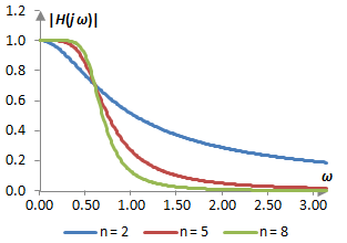
Butterworth aimed at designing a filter that had both a good stop band attenuation as well as uniform (flat) magnitude response in the pass band. The following is a slight modification the desired magnitude response used in the original Butterworth paper.

$$|H(j\omega)|=\frac{G}{\sqrt{1+(\frac{\omega}{\omega_c})^{2n}}}$$

Assuming that ω and ω_c are normalized frequencies and hence span the frequency spectrum between 0 and π, a plot of this desired magnitude response with ω_c = 0.6 and three different values of n – 2, 5 and 8 – is shown below. This function indeed behaves like the magnitude response of a low pass filter – one that has a cutoff frequency of ω_c and one that improves with larger n.

We note that the Butterworth magnitude response is monotonically decreasing. The first derivative of the Butterworth magnitude response is

$$|H(j\omega)|'=((1+(\frac{\omega}{\omega_c})^{2n})^{-\frac{1}{2}})'=-n\,\omega^{2n-1}|H(j\omega)|^3$$

This derivative is always negative, as the magnitude response and the frequency are always positive. This means that the magnitude response always decreases and has no ripples.

If we continue taking the derivative of the magnitude response we will note that at ω = 0, all derivatives up to the 2n-th derivative are zero. Thus, this filter is said to have maximally flat magnitude response.

The magnitude response

$$|H(j\omega)|=\frac{G}{\sqrt{1+(\frac{\omega}{\omega_c})^{2n}}}=\frac{G}{\sqrt{1+(\frac{\omega^2}{\omega_c^2})^n}}$$

means that the squared transfer function, with s = j ω, should translate to something like

$$H(s)^2=\frac{G^2}{1+(\frac{-s^2}{\omega_c^2})^n}$$

We can rewrite the squared transfer function expression by solving for the roots of the denominator

$$1+(\frac{-s^2}{\omega_c^2})^n=0$$ $$s=\pm \omega_c \,e^{\frac{j(2k-1)\pi}{2n}}, \, k=1,2,...,2n$$ $$H(s)^2=G^2 \prod_{k=1}^{2n} \frac{1}{s-s_k}$$

For example, when n = 2, the denominator of the squared magnitude response produces four evenly spaced roots

$$s_1=\omega_c \, e^{j\frac{\pi}{4}}=\omega_c (\cos(\frac{\pi}{4})+j \, \sin(\frac{\pi}{4}))=(\frac{1}{\sqrt{2}}+j \frac{1}{\sqrt{2}})\omega_c$$ $$s_2=\omega_c \, e^{j\frac{3\pi}{4}}=(-\frac{1}{\sqrt{2}}+j \frac{1}{\sqrt{2}})\omega_c$$ $$s_3=-\omega_c \, e^{j\frac{\pi}{4}}=(-\frac{1}{\sqrt{2}}-j \frac{1}{\sqrt{2}})\omega_c$$ $$s_4=-\omega_c \, e^{j\frac{3\pi}{4}}=(\frac{1}{\sqrt{2}}-j \frac{1}{\sqrt{2}})\omega_c$$

Note that s₁ and s₄ are complex conjugates and s₂ and s₃ are complex conjugates. Thus, when n = 2

$$H(s)^2=\frac{G^2}{(s-s_1)(s-s_2)(s-s_3)(s-s_4)}$$

and

$$H(s)=\frac{G}{(s-s_a)(s-s_b)}$$

where s_a and s_b are some combination of two of the four roots. (Usually, rather than writing H(s)², we write H(s)H(-s). We assume that the magnitude response is symmetric around zero, which has benefits. Since Fourier transforms, Laplace transforms, and Z transforms employ sine and cosine functions, which are respectively negative (sin(x) = -sin(-x)) and symmetric (cos(x) = cos(-x)) functions, taking the inverse transform of a symmetric desired magnitude response typically allows us to produce a filter of real valued coefficients. Such filter is sometimes referred to as a "zero phase" filter. That is, the impact of such a filter on the signal depends on the frequency of the signal and not on the phase.)

If we are familiar with IIR filters, we would obviously take the two roots with negative real parts, as that ensures that the filter is stable (s₂ and s₃ above). The following is a somewhat simple explanation of why this makes sense.

Since we prefer a transfer function that depends on the frequency and not on the phase, we would pick, again, s_a and s_b such that the transfer function becomes one of real coefficients. This means taking two complex conjugate roots. We can also note that the complex pairs s₁ and s₄ and s₂ and s₃ produce similar, but slightly different Z transform functions, denoted by +/- in the function below.

$$H(z)=\frac{-\sqrt{2}\omega_c \, \sin(\frac{\omega_c}{\sqrt{2}}) e^{\pm\frac{\omega_c}{\sqrt{2}}}z^{-1}}{1-2\,\cos(\frac{\omega_c}{\sqrt{2}})e^{\pm\frac{\omega_c}{\sqrt{2}}}z^{-1}+e^{\pm \sqrt{2}\omega_c}z^{-2}}$$

In fact, the pair s₁ and s₄ produces

$$H(z)=\frac{-0.533888z^{-1}}{1-2.785910z^{-1}+2.33606z^{-2}}$$

This filter is unstable. If we put a simple wave through it, the sampled values of output will begin increasing indefinitely, which is a matter of simply taking any simple sine or cosine wave and trying it out.

The stability / instability of these two filters can also be explained by saying that a stable system is one that produces reasonable (bound) response to any reasonable (bound) input. The Laplace transform of such system must be bound. Since in practice we only work with nonnegative amplitudes, we want a Laplace transform transfer function be bound for all s for which σ = Re(s) ≥ 0. If the transfer function has denominator roots (poles) where it is not bound, these roots must have negative real parts.

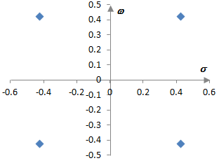
The second order low pass Butterworth filter has four potential poles as described above. Those are shown on here for ω_c = 0.6 in the complex s plane. The stable filter can be created by taking the two poles with negative real parts, which are the ones in the left half plane.