The Kaiser window coefficients are given by the following formula
$$a(k)=\frac{I_0(\pi\,\alpha \sqrt{1-(\frac{2k}{N-1}-1)^2}\,)}{I_0(\pi\,\alpha)}$$
where N is the length of the filter, k = 0, 1, …, N – 1, α is any real number, and I0 is the zero order modified Bessel function of the first kind.
Computing the Kaiser window
The modified Bessel function of the first kind (the hyperbolic Bessel function) is defined as follows.
$$I_{\beta}(x)=\sum_{n=0}^{\infty}\frac{1}{n!\,\Gamma(n+\beta+1)}(\frac{x}{2})^{2n+\beta}$$
where β is the order of the function and Γ is the generalized factorial.
Note that for any positive integer n, Γ(n) = (n – 1)!. Then at β = 0, Γ(n + β + 1) = (n + 0 + 1 – 1)! = n!. This means that the zero order modified Bessel function of the first kind is simply
$$I_0(x)=\sum_{n=0}^{\infty}(\frac{1}{n!})^2(\frac{x}{2})^{2n}$$
The sum converges and we can be approximate for any x, if we take the first few terms, say
$$I_0(x)=\sum_{n=0}^{M}(\frac{1}{n!})^2(\frac{x}{2})^{2n}$$
The Kaiser window itself, if we rewrite the numerator and denominator as per the discussion above, can be written as follows.
$$a(k)=\frac{\sum_{n=0}^{\infty}(\frac{1}{n!})^2(\frac{\pi\, \alpha \sqrt{1-(\frac{2k}{N-1}-1)^2}}{2})^{2n}}{\sum_{n=0}^{\infty}(\frac{1}{n!})^2(\frac{\pi\, \alpha}{2})^{2n}}$$
As before, both sums converge and can be approximated by taking the first few terms.
An example Kaiser window
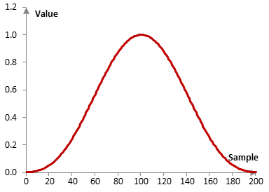
Consider a finite impulse response (FIR) low pass filter of length N = 201. The following is the Kaiser window with α = 3 and M = 4.
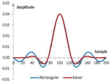
Given a sampling frequency of 2000 Hz and a filter cutoff frequency of 40 Hz, the impulse response of the filter with a rectangular window (with no window) and with the Kaiser window is as follows.
The magnitude response of the same filter is shown on the graph below.
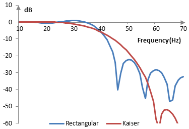
As the absolute value of α increases, the windowed filter produces a larger transition band, but better stop band attenuation. As |α| decreases, the filter has a smaller transition band and worse stop band attenuation. At α = 0 the Kaiser window becomes a rectangular window.
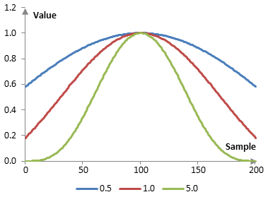
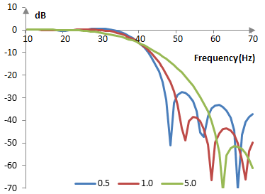
The Kaiser window with N = 201 for three different values of α (0.5, 1, and 5) is shown below.
The following are the magnitude responses of these windows, applied to a filter with a cutoff frequency of 40 Hz, given a sampling frequency of 2000 Hz.
Measures for the Kaiser window
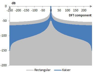
The following is a comparison of the discrete Fourier transform of the Kaiser window (α = 1.0) and the rectangular window.
The Kaiser window measures are as follows.
| α | 0.5 | 1.0 | 5.0 |
| Coherent gain | 0.85 | 0.67 | 0.42 |
| Equivalent noise bandwidth | 1.02 | 1.15 | 1.76 |
| Processing gain | -0.10 dB | -0.62 dB | -2.44 dB |
| Scalloping loss | -3.31 dB | -2.42 dB | -1.05 dB |
| Worst case processing loss | -3.41 dB | -3.04 dB | -3.49 dB |
| Highest sidelobe level | -16.6 dB | -24.6 dB | -38.6 dB |
| Sidelobe falloff | -6.4 dB / octave, -21.2 dB / decade | -7.3 dB / octave, -24.2 dB / decade | -15.5 dB / octave, -51.6 dB / decade |
| Main lobe is -3 dB | 0.96 bins | 1.10 bins | 1.68 bins |
| Main lobe is -6 dB | 1.30 bins | 1.52 bins | 2.34 bins |
| Overlap correlation at 50% overlap | 0.479 | 0.370 | 0.080 |
| Amplitude flatness at 50% overlap | 0.895 | 0.829 | 0.691 |
| Overlap correlation at 75% overlap | 0.794 | 0.783 | 0.559 |
| Amplitude flatness at 75% overlap | 0.974 | 0.958 | 0.991 |
See also:
Window
Add new comment