The sidelobe falloff of a window is the rate at which the side lobes of the discrete Fourier transform of the window decrease in magnitude.
The approach to computing sidelobe falloff for the windows in this site is simplistic. Assuming the discrete Fourier transform of the window is adjusted so that the main lobe of the transform peaks at 0 dB, the sidelobe falloff is computed as the ratio of the peak of the last lobe (in decibels) over the number of octaves or decades in the transform. The sidelobe falloff is thus measured in dB per octave or in dB per decade. The octaves or decades in the discrete Fourier transform are computed as log2(N/2) or log10(N/2), where N is the length of the transform.
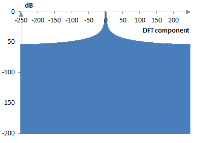
For example, the following is the discrete Fourier transform of 500 points of the rectangular window.

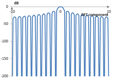
If we zoom in and compute the transform also of points in between the transform components, we will see the lobes. The following graph shows the main lobe and several side lobes of the transform.

The last component, which is visible in the first graph above, but falls outside of the second graph, has a peak of -53.9 dB. The sidelobe falloff of the rectangular window then is -53.9 / log2(250) = -6 dB / oct or -53.9 / log10(250) = -20 dB / dec.
Sidelobe falloff for common windows
The following is the sidelobe falloff of some common windows (in dB per octave, dB per decade, with the window definitions on this site).
| Bartlett-Hann | -12.7, -42.3 |
| Blackman Exact Blackman Generalized Blackman α = 0.05 α = 0.20 α = 0.35 |
-21.6, -71.7 -10.0, -33.3 -20.9, -69.5 |
| Blackman-Harris | -14.4, -48.0 |
| Blackman-Nuttall | -12.7, -42.2 |
| Bohman | -21.4, -71.0 |
| Dolph-Chebychev ω0 = 0.1 ω0 = 0.2 ω0 = 0.3 |
-7.1, -23.5 -7.1, -23.5 -7.1, -23.5 |
| Flat top | -12.1, -40.1 |
| Gaussian σ = 0.3 σ = 0.5 σ = 0.7 Approximate confined Gaussian σ = 0.3 σ = 0.5 σ = 0.7 Generalized normal α = 2 α = 4 α = 6 |
-10.5, -34.8 -7.5, -24.8 -6.7, -22.3 -18.4, -61.1 -7.5, -24.8 |
| Hamming | -7.9, -26.1 |
| Hann | -20.7, -68.9 |
| Hann-Poisson α = 0.3 α = 0.5 α = 0.7 |
-17.4, -57.7 -16.8, -55.9 -16.4, -54.6 |
| Kaiser α = 0.5 α = 1.0 α = 5.0 |
-6.4, -21.2 -7.3, -24.2 -15.5, -51.6 |
| Kaiser-Bessel | -11.8, -39.3 |
| Lanczos | -11.5, -38.3 |
| Nuttall | -23.4, -77.6 |
| Parzen | -7.0, -23.3 |
| Planck-taper ε = 0.2 ε = 0.4 ε = 0.5 |
-27.4, -90.9 -30.9, -102.6 -30.8, -102.3 |
| Poisson α = 0.2 α = 0.5 α = 0.8 |
-6.1, -20.3 -6.3, -20.8 -6.4, -21.4 |
| Power of cosine α = 1.0 α = 2.0 α = 3.0 |
-11.2, -37.1 -20.7, -68.9 -21.3, -70.6 |
| Rectangular | -6.0, -20.0 |
| Sine | -11.2, -37.1 |
| Triangular | -11.4, -37.7 |
| Tukey α = 0.3 α = 0.5 α = 0.7 |
-16.3, -54.3 -15.8, -52.6 -15.3, -50.9 |
| Ultraspherical (x0 = 1) μ = 2 μ = 3 μ = 4 |
-10.7, -35.4 -14.6, -48.6 -18.2, -60.5 |
| Welch | -11.0, -36.5 |
Add new comment