For a system with the transfer function H(j ω), the equivalent noise bandwidth is
$$B_N=\frac{1}{2\pi} \int_0^{\infty} |\frac{H(j \, \omega)}{H_{max}}|^2 \,d\omega$$
where Hmax is the maximum value of |H(j ω)|.
The equivalent noise bandwidth may be abbreviated as ENBW or NBW and may also be named "noise equivalent bandwidth".
Note that the ENBW in the equation above is normalized both for the maximum value of H as well as for the interval spanned by ω of length 2 π. Thus, for example, an all pass filter with a gain of 1 should have ENBW = 1.
Equivalent noise bandwidth for filters
The equation above measures the amount of noise power that the system passes (the square on |H| implies power, see Decibel (dB); the term "noise" makes sense as we are concerned with the whole frequency spectrum). ENBW thus measures the noise power that is accumulated in the magnitude response of the filter, as explained below.
Most filters do not allow all frequencies of the signal through with the same power. A low pass filter, for example, will pass lower frequencies with minor changes in magnitude and hence power, but will reduce the magnitude / power of higher frequencies. Whatever power a practical low pass filter passes, there is an ideal low pass filter with a square magnitude response that would pass the same power as shown in the graph below.
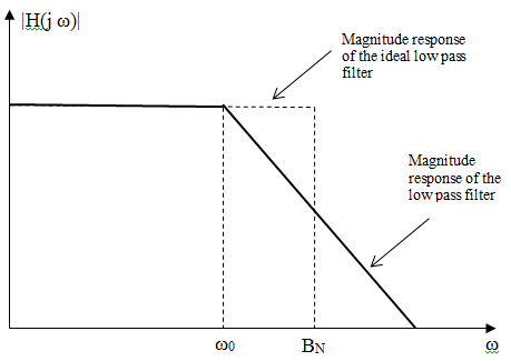
The bandwidth BN of that ideal filter is the equivalent noise bandwidth.
Note that BN increases as the cutoff frequency of the low pass filter increases. Hence, on occasion, we use the ratio BN / ω0 rather than just the bandwidth BN. This ratio becomes smaller as the low pass filter improves, as with a higher length or higher cutoff frequencies for finite impulse response filters or with higher order for infinite impulse response filters.
Note that, with practical filters, the frequency ω0 does not exist. There is no specific frequency where the magnitude responses changes from a flat, horizontal one to a decreasing one. Typically, ω0 is chosen as the frequency at which the magnitude response of the filter reaches -3 dB.
For example, the simplest first order Butterworth filter is
$$H(s)=\frac{1}{1+\frac{s}{\omega_c}}=\frac{1}{1+j \frac{\omega}{\omega_c}}$$
where ωc is the cutoff frequency. The magnitude response of this filter is
$$|H(j\omega)|=\frac{\omega_c}{\sqrt{\omega_c^2+\omega^2}}$$
Since the magnitude response of the Butterworth filter is monotonically decreasing, Hmax = H(0) = 1. The equivalent noise bandwidth is
$$B_N=\frac{1}{2\pi} \int_0^{\infty} \frac{\omega_c^2}{\omega_c^2+\omega^2} \,d\omega=\frac{\pi}{2} \frac{\omega_c}{2\pi} \approx 1.57 \frac{\omega_c}{2\pi}$$
Thus, the ENBW is proportional to the normalized cutoff frequency. Note that the magnitude response at the cutoff frequency is
$$|H(j\omega)|=\frac{\omega_c}{\sqrt{\omega_c^2+\omega_c^2}}=\frac{1}{\sqrt{2}} \approx -3 db$$
The ENBW relative to the -3 dB frequency is 1.57.
Equivalent noise bandwidth for windows
Consider a window w(k) defined in discrete time and applied to a finite impulse response filter. If we treat this window as a filter, then its equivalent noise bandwidth is
$$B_N=\sum_{n=0}^N |\frac{H(\omega_n)}{H_{max}}|^2$$
By Parseval's theorem
$$B_N=\frac{1}{|H_{max}|^2} \sum_{n=0}^{N-1} |H(\omega_n)|^2=\frac{N}{|H_{max}|^2} \sum_{k=0}^{N-1} |w(k)|^2$$
For a typical window, Hmax occurs at ω = 0 and is the 0th component of the discrete Fourier transform
$$|H_{max}|^2=(\sum_{k=0}^{N-1} w(k))^2$$
and so
$$B_N=\frac{N \sum_{k=0}^{N-1} |w(k)|^2}{(\sum_{k=0}^{N-1} w(k))^2}$$
For the rectangular window, for example,
$$B_N=\frac{N N}{N^2}=1$$
For other common windows, BN > 1. The magnitude response of the Hamming window, if the window is treated as a filter, is shown on the graph below (computed with some limited precision). This is a window of length N = 201 points. This graph covers a portion of the frequency spectrum, which is from 0 to π. Also, the window peaks at 1 and is not scaled to ensure that, when used as a filter, it results in a magnitude response at 0 of 1.
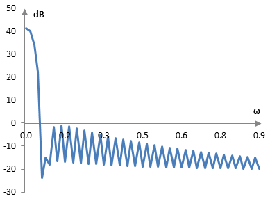
The equivalent noise bandwidth of this winow is BN = 1.37. (The equivalent noise bandwidth becomes smaller with Hamming windows of larger length; it will be closer to 1.36).
A windowed filter is the product f(k) w(k) of the standard filter f(k) and the window w(k). According to the convolution theorem, the Fourier transform of this product is the convolution of the Fourier transforms.
$$F(f \,w)=F(f) * F(w)$$
Thus, the magnitude response of the window acts as a filter on the magnitude response of the filter before the window.
For typical windows, the smaller BN is, the more the magnitude response of this window will show a steeper decline from |H(0)| to the side lobes. This means that the magnitude response of a typical window will resemble more closely an impulse. The impact of the magnitude response of the window (the filter in the convolution above) over the magnitude response of the standard filter will be like that of an all pass filter. A standard finite impulse response all pass filter is an impulse. The smaller the equivalent noise bandwidth, the closer the window is to the rectangular window. For example, the Tukey window, as defined in this site, approximates the rectangular window as the window's parameter α becomes larger. When α becomes larger, the ENBW of the Tukey window approaches 1.
Equivalent noise bandwidth for common windows
The following is the equivalent noise bandwidth of some common windows (with the window definitions on this site).
| Bartlett-Hann | 1.46 |
| Blackman Exact Blackman Generalized Blackman α = 0.05 α = 0.20 α = 0.35 |
1.73 1.70 1.56 |
| Blackman-Harris | 2.01 |
| Blackman-Nuttall | 1.98 |
| Bohman | 1.79 |
| Dolph-Chebychev ω0 = 0.1 ω0 = 0.2 ω0 = 0.3 |
1.80 2.33 2.72 |
| Flat top | 3.78 |
| Gaussian σ = 0.3 σ = 0.5 σ = 0.7 Approximate confined Gaussian σ = 0.3 σ = 0.5 σ = 0.7 Generalized normal α = 2 α = 4 α = 6 |
1.89 1.23 1.08 1.89 1.23 |
| Hamming | 1.36 |
| Hann | 1.50 |
| Hann-Poisson α = 0.3 α = 0.5 α = 0.7 |
1.57 1.61 1.66 |
| Kaiser α = 0.5 α = 1.0 α = 5.0 |
1.02 1.15 1.76 |
| Kaiser-Bessel | 1.80 |
| Lanczos | 1.30 |
| Nuttall | 2.03 |
| Parzen | 1.12 |
| Planck-taper ε = 0.2 ε = 0.4 ε = 0.5 |
1.19 1.46 1.63 |
| Poisson α = 0.2 α = 0.5 α = 0.8 |
1.00 1.02 1.05 |
| Power of cosine α = 1.0 α = 2.0 α = 3.0 |
1.24 1.50 1.74 |
| Rectangular | 1.00 |
| Sine | 1.24 |
| Triangular | 1.34 |
| Tukey α = 0.3 α = 0.5 α = 0.7 |
1.33 1.22 1.13 |
| Ultraspherical (x0 = 1) μ = 2 μ = 3 μ = 4 |
1.18 1.39 1.57 |
| Welch | 1.20 |
Add new comment