When the Fourier transform is used to analyze the frequency content of signals, the signal is often windowed to make the Fourier transform more precise. For similar reasons, the signal segments over which the Fourier transform is used are often selected to overlap. Depending on how the overlap is chosen, the overlapping windows change the amplitude of the signal. This change is different for different points of the signal.
The amplitude flatness of a window is the ratio of the minimum to maximum amplitude that is applied to samples of the signal during the windowing of the signal.
The following graph for example shows six Hann windows of length 50 points that overlap by 40% (by 20 samples). The total amplitude that this window configuration will apply to each sample of the signal varies between 0.69 in the middle between windows and 1 at the peak of each window (the dotted line below; this total amplitude is simply the sum of the window values over the timeline).
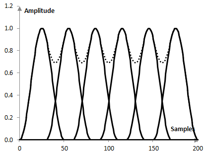
Thus, the amplitude flatness of the Hann window at 40% overlap is 0.69. This number will increase as the overlap increases.
Optimal overlap
With the Hann window specifically, when the overlap is 50%, the amplitude flatness becomes 1. In other words, the total weight applied by the windows to each sample of the signal is the same (it is 1). Incidentally, with this overlap, the difference between the amplitude flatness and the overlap correlation of the Hann window is the largest. The 50% overlap then is sometimes called the "optimal overlap" for the Hann window, in the sense that it gets a maximum amplitude flatness for minimum overlap correlation. The maximum amplitude flatness means that the amplitude of all samples is the same (for the Hann window, almost the same for most other windows) and so no sample is less important in the spectral analysis – no data is lost. The minimum overlap correlation means no unnecessary overlap and computational intensity of the spectral analysis. The "optimal overlap" then is the overlap that achieves a relatively small loss of data for relatively few computations. The type of overlap where the amplitude flatness becomes 1usually does not exist with other windows. The optimal overlap, however, can still be defined in the same way.
Power flatness
The power flatness of a window is defined in the same way, but instead of summing the values of the overlapping windows, it sums the squared values of the overlapping windows. The power flatness is a measure that is more appropriate for signals that are less similar to sinusoids and more resembling noise.
Amplitude flatness for common windows
The following is the amplitude flatness of some common windows (at 50% overlap, at 75% overlap, with the window definitions on this site).
| Bartlett-Hann | 1.000, 1.000 |
| Blackman Exact Blackman Generalized Blackman α = 0.05 α = 0.20 α = 0.35 |
0.680, 1.000 0.695, 1.000 0.900, 1.000 |
| Blackman-Harris | 0.435, 1.000 |
| Blackman-Nuttall | 0.454, 1.000 |
| Bohman | 0.637, 0.982 |
| Dolph-Chebychev ω0 = 0.1 ω0 = 0.2 ω0 = 0.3 |
0.272, 0.914 0.154, 0.579 0.127, 0.377 |
| Flat top | -0.110, 0.938 |
| Gaussian σ = 0.3 σ = 0.5 σ = 0.7 Approximate confined Gaussian σ = 0.3 σ = 0.5 σ = 0.7 Generalized normal α = 2 α = 4 α = 6 |
0.497, 0.998 0.936, 0.973 0.878, 0.969 0.498, 0.998 0.936, 0.973 |
| Hamming | 1.000, 1.000 |
| Hann | 1.000, 1.000 |
| Hann-Poisson α = 0.3 α = 0.5 α = 0.7 |
0.861, 0.977 0.779, 0.960 0.705, 0.942 |
| Kaiser α = 0.5 α = 1.0 α = 5.0 |
0.895, 0.974 0.829, 0.958 0.691, 0.991 |
| Kaiser-Bessel | 0.608, 1.000 |
| Lanczos | 0.785, 0.947 |
| Nuttall | 0.423, 1.000 |
| Parzen | 0.869, 0.966 |
| Planck-taper ε = 0.2 ε = 0.4 ε = 0.5 |
0.500, 0.860 0.672, 0.923 1.000, 1.000 |
| Poisson α = 0.2 α = 0.5 α = 0.8 |
0.995, 0.999 0.970, 0.992 0.925, 0.980 |
| Power of cosine α = 1.0 α = 2.0 α = 3.0 |
0.707, 0.924 1.000, 1.000 0.707, 0.990 |
| Rectangular | 1.000, 1.000 |
| Sine | 0.707, 0.924 |
| Triangular | 1.000, 1.000 |
| Tukey α = 0.3 α = 0.5 α = 0.7 |
0.616, 0.978 0.500, 1.000 0.500, 0.776 |
| Ultraspherical (x0 = 1) μ = 2 μ = 3 μ = 4 |
0.684, 0.914 0.859, 0.982 0.908, 0.992 |
| Welch | 0.670, 0.910 |
Comments
Formula?
Is there a formula to calculate this?
The formula depends on the window and overlap
This is just a ratio of the highest and lowest point of a window or several windows summed up. The formula is the formula of the window or the sum of several windows, depending on how much the windows overlap. So, you cannot have a single formula here. It will change with the window and with the overlap.
Add new comment