The overlap correlation of a window w(k) is computed with the formula
$$OC(r)=\frac{\sum_{k=0}^{rN-1} w(k)\,w(k+(1-r)N)}{\sum_{k=0}^{N-1}(w(k))^2}$$
where N is the length of the window and r is the amount of overlap, 0 < r ≤ 1.
When a signal is analyzed with the Fourier transform, we often take the Fourier transform of overlapping segments of the signal. This has advantages. For example, it can be shown that with overlapping segments the Fourier transform is more precise in determining the true frequency and phase of the signal. A second advantage of feeding overlapping segments to the Fourier transform is that, if a window is applied to the signal before the Fourier transform, then the loss of data is smaller with the overlap. The loss of data occurs because the sides of the window depress the signal amplitudes.
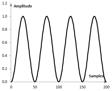
In the following graph, for example, the Fourier transform of 50 points is taken four times over 200 samples, over four non-overlapping segments, and the Hann window is applied before the transform. The Hann window will essentially zero out the points of the signal at sample 0, 50, 100, 150, and 200 and significantly decrease the contributions of points around these samples to the signal.
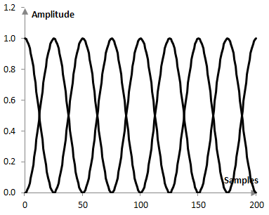
This can be avoided, if we use overlapping segments. With the Hann window, in fact, the 50% overlap case has the nice property that the sum of the applied weight to each sample of the signal is exactly 1 (an overlap that produces such a result does not typically exist for other windows). The problem with larger overlaps is that the Fourier transform, which is computationally intensive, has to be used many more times. While the Fourier transform of 50 components on 200 samples with no overlap will be computed four times, with 50% overlap, it will be computed 8 times, as in the figure below.
In addition, two neighboring transforms produce similar data. The larger the overlap, the closer the transform values are. In this sense, too much overlap produces additional computation for no additional benefit.
The overlap correlation is the degree of correlation produced by the values of neighboring transforms. For example, the overlap correlation of the Hann window with r = 0.5 is 0.165. With larger overlap, this correlation is larger. At r = 0.75, the overlap correlation is 0.658. (See Amplitude flatness for a discussion of the "optimal overlap").
Overlap correlation for common windows
The following is the overlap correlation of some common windows (at 50% overlap, at 75% overlap, with the window definitions on this site).
| Bartlett-Hann | 0.186, 0.674 |
| Blackman Exact Blackman Generalized Blackman α = 0.05 α = 0.20 α = 0.35 |
0.089, 0.565 0.099, 0.576 0.143, 0.635 |
| Blackman-Harris | 0.037, 0.459 |
| Blackman-Nuttall | 0.041, 0.469 |
| Bohman | 0.073, 0.544 |
| Dolph-Chebychev ω0 = 0.1 ω0 = 0.2 ω0 = 0.3 |
0.155, 0.440 0.120, 0.261 0.102, 0.201 |
| Flat top | -0.015, 0.044 |
| Gaussian σ = 0.3 σ = 0.5 σ = 0.7 Approximate confined Gaussian σ = 0.3 σ = 0.5 σ = 0.7 Generalized normal α = 2 α = 4 α = 6 |
0.060, 0.498 0.311, 0.755 0.431, 0.801 0.059, 0.497 0.311, 0.755 |
| Hamming | 0.233, 0.706 |
| Hann | 0.165, 0.658 |
| Hann-Poisson α = 0.3 α = 0.5 α = 0.7 |
0.140, 0.631 0.124, 0.612 0.110, 0.591 |
| Kaiser α = 0.5 α = 1.0 α = 5.0 |
0.479, 0.794 0.370, 0.783 0.080, 0.559 |
| Kaiser-Bessel | 0.072, 0.537 |
| Lanczos | 0.272, 0.733 |
| Nuttall | 0.035, 0.452 |
| Parzen | 0.393, 0.792 |
| Planck-taper ε = 0.2 ε = 0.4 ε = 0.5 |
0.392, 0.721 0.202, 0.666 0.115, 0.614 |
| Poisson α = 0.2 α = 0.5 α = 0.8 |
0.497, 0.773 0.480, 0.794 0.450, 0.799 |
| Power of cosine α = 1.0 α = 2.0 α = 3.0 |
0.317, 0.755 0.165, 0.568 0.084, 0.565 |
| Rectangular | 0.500, 0.752 |
| Sine | 0.317, 0.755 |
| Triangular | 0.248, 0.718 |
| Tukey α = 0.3 α = 0.5 α = 0.7 |
0.272, 0.710 0.362, 0.727 0.430, 0.738 |
| Ultraspherical (x0 = 1) μ = 2 μ = 3 μ = 4 |
0.359, 0.772 0.223, 0.702 0.138, 0.632 |
| Welch | 0.345, 0.765 |
Add new comment