The ultraspherical window coefficients are given by the formula
$$a_0(m)=\frac{1}{N}(C_{N-1}^\mu (x_0)+2 \sum_{n=1}^{\frac{N-1}{2}} (C_{N-1}^\mu (x_0 \cos(\frac{\pi \, n}{N}) \cos(\frac{2 \pi \, n \, m}{N}))))$$ $$m=-\frac{N-1}{2}, -\frac{N-1}{2}+1, …, \frac{N-1}{2}$$ $$a(k)=\frac{a_0(k-\frac{N-1}{2})}{a_0(0)}, k=0, 1, …, N-1$$
where N is the length of the filter, μ and x0 are constants that control the speed with which the lobes of the window decay (usually μ ≥ 1 and x0 ≥ 1), and CμN are the ultraspherical polynomials, also called Gegenbauer polynomials, defined by the recursive relationship
$$C_0^\mu (x)=1$$ $$C_1^\mu (x)=2\,\mu \, x$$ $$C_n^\mu (x)=\frac{1}{n} (2(n+\mu-1)x\,C_{n-1}^\mu (x)-(n+2\,\mu-2) C_{n-2}^\mu (x))$$
a0(k) is a window that is symmetric around the origin and does not peak at 1. a(k) shifts this window to the right by (N – 1) / 2 to k=0, 1, …, N – 1 and scales it so that it peaks at 1. Note that there are a number of other equivalent definitions of the ultraspherical polynomials. Note also that the primary difficulty with computing this window is computing the ultraspherical polynomials, because they may involve very large numbers.
a0(k) is actually the inverse discrete Fourier transform of the desired magnitude response
$$H(k)=C_{N-1}^\mu (x_0 \cos(\frac{\pi\,k}{N}))$$
for k = 0, 1, …, (N – 1) /2.
An alternative and equivalent definition of the window uses
$$a_0(k)=b_{\frac{N-1}{2}-|k|, N-1}^\mu (x_0)$$ $$b_{m,n}^\mu (x_0)=\frac{2\,\mu \, x_0^n}{n-m} (\begin{matrix} \mu+n-m-1 \\ n-m-1 \end{matrix}) \sum_{i=0}^m ((\begin{matrix} \mu+m-1 \\ m-i \end{matrix}) (\begin{matrix} n-m \\ i \end{matrix}) (1-x_0^{-2})^i)$$ $$(\begin{matrix} n \\ m \end{matrix}) = \frac{n!}{m! (n-m)!}$$
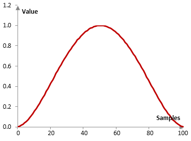
Consider a finite impulse response (FIR) low pass filter of length N = 101. The following is the ultraspherical window with μ = 3 and x0 = 1.
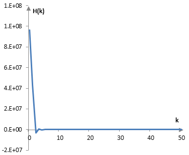
The following is the corresponding desired magnitude response (prior to scaling).
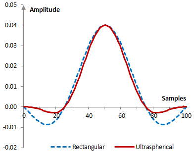
Given a sampling frequency of 2000 Hz and a filter cutoff frequency of 40 Hz, the impulse response of the filter with a rectangular window (with no window) and with the ultraspherical window above is as follows.
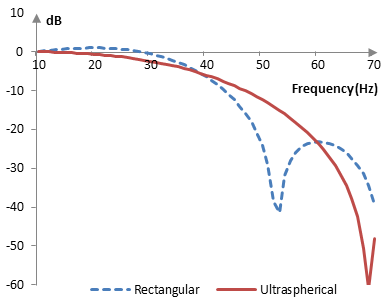
The magnitude response of the same filter is shown on the graph below.
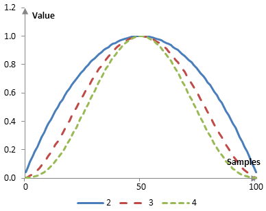
With larger μ, the side lobes of the window decrease faster and the magnitude response of the corresponding filter shows a larger transition band and better stop band attenuation. The following is the ultraspherical window at x0 = 1 and three different values of μ (2, 3, and 4).
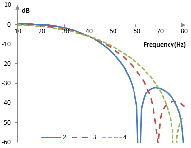
The corresponding magnitude responses for the same low pass filter used in the example above are as follows.
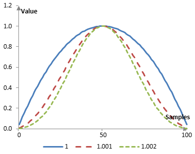
The impact of x0 is similar. The following is the ultraspherical window at μ = 2 and three values of x0 (1, 1.001, and 1.002).
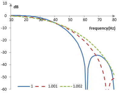
The corresponding magnitude responses, computed with the same low pass filter used in the examples above, are as follows.
Measures for the ultraspherical window
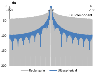
The following is a comparison of the discrete Fourier transform of the ultraspherical window (μ = 3, x0 = 1) and the rectangular window.
The ultraspherical window measures are as follows (x0 = 1; μ = 2, 3, and 4).
| μ | 2 | 3 | 4 |
| Coherent gain | 0.68 | 0.55 | 0.48 |
| Equivalent noise bandwidth | 1.18 | 1.39 | 1.57 |
| Processing gain | -0.71 dB | -1.42 dB | -1.96 dB |
| Scalloping loss | -2.32 dB | -1.66 dB | -1.30 dB |
| Worst case processing loss | -3.02 dB | -3.08 dB | -3.26 dB |
| Highest sidelobe level | -21.3 dB | -27.7 dB | -33.3 dB |
| Sidelobe falloff | -10.7 dB / octave, -35.4 dB / decade | -14.6 dB / octave, -48.6 dB / decade | -18.2 dB / octave, -60.5 dB / decade |
| Main lobe is -3 dB | 1.14 bins | 1.34 bins | 1.50 bins |
| Main lobe is -6 dB | 1.56 bins | 1.84 bins | 2.08 bins |
| Overlap correlation at 50% overlap | 0.359 | 0.223 | 0.138 |
| Amplitude flatness at 50% overlap | 0.684 | 0.859 | 0.908 |
| Overlap correlation at 75% overlap | 0.772 | 0.702 | 0.632 |
| Amplitude flatness at 75% overlap | 0.914 | 0.982 | 0.992 |
See also:
Window
Add new comment