The Gaussian window coefficients are given by the following formula
$$a(k)=e^{-0.5 (\frac{k-M}{\sigma \, M})^2}$$
where N is the length of the filter, M = (N – 1) / 2, k = 0, 1, …, N – 1, and σ > 0.
An example Gaussian window
Consider a finite impulse response (FIR) low pass filter of length N = 201. The following is the Gaussian window with σ = 0.5.
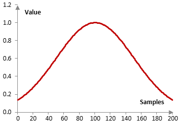
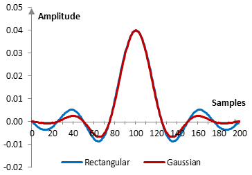
Given a sampling frequency of 2000 Hz and a filter cutoff frequency of 40 Hz, the impulse response of the filter with a rectangular window (with no window) and with the Gaussian window is as follows.
The magnitude response of the same filter is shown on the graph below.
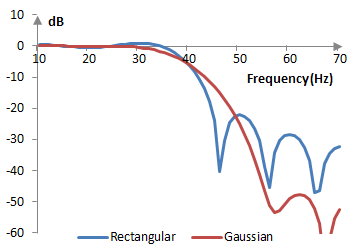
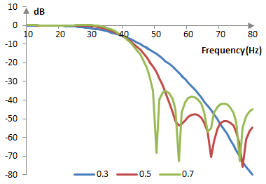
As the parameter σ becomes larger, the transition band of the window decreases and its stop band attenuation becomes worse. As σ approaches infinity, the Gaussian window approaches a rectangular window. If, on the other hand, σ approaches zero, the windowed Gaussian filter approaches an all pass filter.
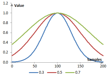
The following is the Gaussian window with N = 201 and at three different values of σ (0.3, 0.5, and 0.7).
The magnitude response of a filter at these values of σ, given a sampling frequency of 2000 Hz and a cutoff frequency of 40 Hz, is shown below.
Measures for the Gaussian window
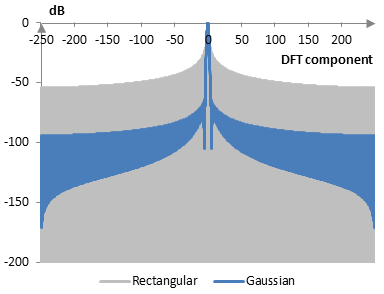
The following graph shows the discrete Fourier transform of the Gaussian window with σ = 0.3 against the discrete Fourier transform of the rectangular window.
The measures of the Gaussian window are as follows.
| σ | 0.3 | 0.5 | 0.7 |
| Coherent gain | 0.37 | 0.60 | 0.74 |
| Equivalent noise bandwidth | 1.89 | 1.23 | 1.08 |
| Processing gain | -2.76 dB | -0.91 dB | -0.32 dB |
| Scalloping loss | -0.95 dB | -2.12 dB | -2.84 dB |
| Worst case processing loss | -3.71 dB | -3.04 dB | -3.16 dB |
| Highest sidelobe level | -64.3 dB | -32.0 dB | -20.9 dB |
| Sidelobe falloff | -10.5 dB / octave, -34.8 dB / decade | -7.5 dB / octave, -24.8 dB / decade | -6.7 dB / octave, -22.3 dB / decade |
| Main lobe is -3 dB | 1.78 bins | 1.18 bins | 1.02 bins |
| Main lobe is -6 dB | 2.50 bins | 1.64 bins | 1.42 bins |
| Overlap correlation at 50% overlap | 0.060 | 0.311 | 0.431 |
| Amplitude flatness at 50% overlap | 0.497 | 0.936 | 0.878 |
| Overlap correlation at 75% overlap | 0.498 | 0.755 | 0.801 |
| Amplitude flatness at 75% overlap | 0.998 | 0.973 | 0.969 |
Approximate confined Gaussian window
The Gaussian window above is actually an approximate confined Gaussian window. A more general approximation of the latter is defined by
$$a(k)= G(k) - \frac{G(-\frac{1}{2})(G(k+N)+G(k-N))}{G(-\frac{1}{2}+N)+G(-\frac{1}{2}-N)}$$ $$G(k)=e^{-0.5 (\frac{k-M}{\sigma \, M})^2}$$
A comparison of the Gaussian and confined Gaussian windows for N = 201 and σ = 0.5 is shown below.
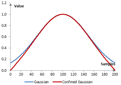
Note that the confined Gaussian window does not necessarily peak at 1 in the middle.
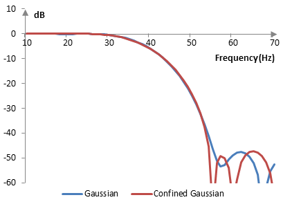
The corresponding magnitude responses, with the same low pass filter used above, are shown on the graph below.
Measures for the approximate confined Gaussian window
The measures of the approximate confined Gaussian window at three values of σ (0.3, 0.5, and 0.7) are as follows.
| σ | 0.3 | 0.5 | 0.7 |
| Coherent gain | 0.37 | 0.57 | 0.61 |
| Equivalent noise bandwidth | 1.89 | 1.32 | 1.24 |
| Processing gain | -2.77 dB | -1.19 dB | -0.94 dB |
| Scalloping loss | -0.95 dB | -1.85 dB | -2.07 dB |
| Worst case processing loss | -3.71 dB | -3.04 dB | -3.01 dB |
| Highest sidelobe level | -63.6 dB | -30.3 dB | -23.5 dB |
| Sidelobe falloff | -18.4 dB / octave, -61.1 dB / decade | -16.3 dB / octave, -54.3 dB / decade | -16.1 dB / octave, -53.5 dB / decade |
| Main lobe is -3 dB | 1.78 bins | 1.26 bins | 1.20 bins |
| Main lobe is -6 dB | 2.50 bins | 1.76 bins | 1.64 bins |
| Overlap correlation at 50% overlap | 0.059 | 0.261 | 0.313 |
| Amplitude flatness at 50% overlap | 0.498 | 0.841 | 0.720 |
| Overlap correlation at 75% overlap | 0.497 | 0.728 | 0.754 |
| Amplitude flatness at 75% overlap | 0.998 | 0.944 | 0.926 |
Generalized normal window
Another generalization of the Gaussian window is the generalized normal window given by the following formula.
$$a(k)=e^{-0.5 |\frac{k-M}{\sigma \, M}|^{\alpha}}$$
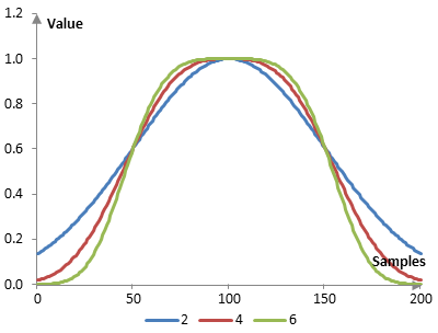
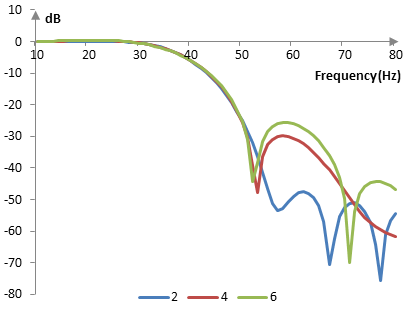
where α > 0 (usually α ≥ 1). At α = 2, the generalized normal window becomes the Gaussian window. As α increases, the top of the generalized normal window becomes flatter, the transition band of the corresponding filter becomes narrower, and its stop band attenuation becomes worse. As α approaches infinity, the generalized normal window approaches the rectangular window.
The following is the generalized normal window at three different values of α (2, 4, and 6) and with σ = 0.5.
The corresponding magnitude responses of the same low pass filter used above with these windows are as follows.
Measures for the generalized normal window
The measures of the generalized normal window with σ = 0.5 and three values of α are as follows.
| α | 2 | 4 | 6 |
| Coherent gain | 0.60 | 0.54 | 0.52 |
| Equivalent noise bandwidth | 1.23 | 1.56 | 1.71 |
| Processing gain | -0.91 dB | -1.94 dB | -2.34 dB |
| Scalloping loss | -2.12 dB | -1.30 dB | -1.09 dB |
| Worst case processing loss | -3.04 dB | -3.24 dB | -3.43 dB |
| Highest sidelobe level | -32.0 dB | -19.7 dB | -16.3 dB |
| Sidelobe falloff | -7.5 dB / octave, -24.8 dB / decade | -13.2 dB / octave, -44.0 dB / decade | -30.8 dB / octave, -102.4 dB / decade |
| Main lobe is -3 dB | 1.18 bins | 1.50 bins | 1.62 bins |
| Main lobe is -6 dB | 1.64 bins | 2.06 bins | 2.22 bins |
| Overlap correlation at 50% overlap | 0.311 | 0.143 | 0.086 |
| Amplitude flatness at 50% overlap | 0.936 | 0.825 | 0.821 |
| Overlap correlation at 75% overlap | 0.755 | 0.635 | 0.582 |
| Amplitude flatness at 75% overlap | 0.973 | 0.948 | 0.900 |
See also:
Gaussian filter, Window
Comments
Older comments
admin, First posted on 2014 04 08
Greg Colvin, 2014 04 08: You say upfront that sigma must be greater than one, but every number called a sigma after that is less than one. So they can't be sigmas, but I don't know what they are.
mic, 2014 04 08: I say that sigma must be greater than zero (not 1).
Greg Colvin, 2014 04 09: Aha, sorry. These are the first sigmas I've ever seen less than 1. I'm used to kernel sizes 2 to 4 times sigma, so I'd expect something closer to 60 for this example. But if I extrapolate your example that far the magnitude response would be a dense mush of lobes. I don't think that can be right, or my filter wouldn't work as well as it does. Time to get out the FFT.
mic, 2014 09 04: Ignore my e-mail with the example. When I think about your comment now, I think you are talking about (sigma * M) and not just sigma. The notation of the "confined" Gaussian window, replaces (sigma * M) with sigma, which makes your comment valid. That is a slightly different window though. I should put that in the writing above. In short, the topic above is correct. You are also correct, but we are talking about two slightly different things.
Greg Colvin, 2014 04 09: The blog came back to life... I wasn't thinking of windows at all, I was thinking of digital filters, where I hadn't seen sigmas that small. But you have me spending a lot of time with a kernel generator and an FFT. Seems the lobing you demonstrate disappears when the kernel is large enough. I can't afford that large a kernel, but am finding that most any of the windows provided with the FFT will remove the lobes. I'm also learning that Gaussian kernels don't have the frequency response I need
..and Gaussian filter
We put a page also for the Gaussian filter. It is linked at the very bottom above. Maybe that page will clear up some of the confusion re constants used in the formulae.
Add new comment